Exploring the CRCNS AA1 and AA2 datasets with deepSTRF

This notebook walks through the deepSTRF dataset API on two closely related auditory neurophysiology datasets:

• CRCNS AA1 (Theunissen et al.,

  2009. — single-unit spike trains from the Field-L and MLd regions of anesthetized zebra finches, responding to conspecific songs and flat ripples.

• CRCNS AA2 (Gill et al., 2006 / Amin et al., 2010) — same species, larger cohort (~500 neurons across Field-L, MLd, OV, CM), three stim classes (conspecific, flat ripples, song ripples).

By the end, you will have seen:

1. How to instantiate a deepSTRF dataset.

2. How the data are stored internally (list-of-lists, NaN-sentinel missingness) — see `data_paradigm.md <../docs/_source/md/data_paradigm.md>`__ for the full design rationale.

3. How to visualize a stimulus spectrogram and its recorded PSTH.

4. How to use the neuron selection API (select_neuron, select_pop_by_nrn_attr, …).

5. How to iterate the dataset with a PyTorch ``DataLoader`` via the batch-collate function.

Data: the AA1 / AA2 archives are auto-downloaded from crcns.org on first use (download=True in the constructor). You’ll need a free CRCNS account — see the setup section below.

Setup — Google Colab

If you’re running on Google Colab, the cell below installs deepSTRF from source. On a local install (pip install -e .) it’s a no-op.

Note on data: AA1 and AA2 are authenticated CRCNS datasets. To auto-download them, set $CRCNS_USERNAME and $CRCNS_PASSWORD (free account at https://crcns.org/) before running the dataset cells. On a local machine that already has the data extracted, it’s picked up from the cache automatically.

import sys
if 'google.colab' in sys.modules:
    !pip install -q git+https://github.com/urancon/deepSTRF.git
    print("deepSTRF installed from GitHub.")
else:
    print("Local environment — assuming deepSTRF is already importable.")

Imports

%matplotlib inline
import matplotlib.pyplot as plt
import torch
from torch.utils.data import DataLoader

from deepSTRF.datasets.audio.crcns_aa1 import CRCNSAA1Dataset
from deepSTRF.datasets.audio.crcns_aa2 import CRCNSAA2Dataset
from deepSTRF.utils.data import neural_collate

# Bin width in ms. Typical choices: 1, 5, 10.
DT_MS = 5

1. Instantiating AA1

The constructor takes a path to the data folder, plus dataset-specific selection arguments (recording area, stimulus type, animal, bin width, …). All stimuli and responses are preprocessed in the constructor so the object is ready for iteration immediately.

aa1 = CRCNSAA1Dataset(
    download=True,
    areas=("Field_L", "MLd"),
    stimuli=("conspecific", "flatrip"),
    dt_ms=DT_MS,
)
aa1

2. How data are stored

deepSTRF datasets are triply ragged — stimulus duration varies, repeat count varies per (stim, neuron), and coverage is sparse (not every neuron heard every stim). They are stored as Python lists of tensors rather than stacked tensors, with NaN as the single channel for encoding missingness.

Core attributes populated by every NeuralDataset subclass:

attribute	shape / structure
self.stims	length-S list; each element is a (1, F, T_s) mel-spectrogram (T varies)
self.responses	length-S list of length-N lists; responses[s][n] is (R_{s,n}, T_s) or (1, 1) NaN
self.stim_meta	length-S list of per-stim dicts, e.g. {"name", "type"}
self.nrn_meta	length-N list of per-neuron dicts, e.g. {"cell_id", "animal_id", "area"}
self.nrn_masks	derived @property: (S, N) bool tensor — True iff (stim, neuron) has data

Let’s confirm all the shapes are consistent with the paradigm.

print(f"S (stimuli)           = {aa1.get_S()}")
print(f"N (neurons)           = {aa1.get_N()}")
print(f"dt                    = {aa1.dt} ms")
print()
print(f"stims[0].shape        = {tuple(aa1.stims[0].shape)}  (1, F, T_0)")
print(f"stim T range          = [{min(s.shape[-1] for s in aa1.stims)}, "
      f"{max(s.shape[-1] for s in aa1.stims)}]  bins")
print()
print(f"responses[0][0] shape = {tuple(aa1.responses[0][0].shape)}")
print(f"stim_meta[0]          = {aa1.stim_meta[0]}")
print(f"nrn_meta[0]    = {aa1.nrn_meta[0]}")
print()
print(f"nrn_masks.shape       = {tuple(aa1.nrn_masks.shape)}, dtype = {aa1.nrn_masks.dtype}")
print(f"nrn_masks valid       = {int(aa1.nrn_masks.sum())} / {aa1.nrn_masks.numel()} "
      f"({100 * aa1.nrn_masks.float().mean().item():.1f}%)")

S (stimuli)           = 30
N (neurons)           = 100
dt                    = 5 ms

stims[0].shape        = (1, 32, 389)  (1, F, T_0)
stim T range          = [330, 501]  bins

responses[0][0] shape = (10, 389)
stim_meta[0]          = {'name': '058767E725C83836F405A97FD7D1E751.wav', 'type': 'conspecific'}
nrn_meta[0]    = {'cell_id': 'gg0304_10_B', 'animal_id': 'gg0304', 'area': 'Field_L'}

nrn_masks.shape       = (30, 100), dtype = torch.bool
nrn_masks valid       = 2960 / 3000 (98.7%)

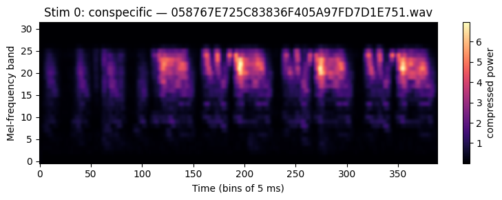
3. Visualizing a stimulus

Stimuli are mel-spectrograms of shape (1, F, T), stored as float tensors.

stim_idx = 0
stim = aa1.stims[stim_idx].squeeze(0)   # (F, T)
meta = aa1.stim_meta[stim_idx]
fig, ax = plt.subplots(figsize=(8, 3))
im = ax.imshow(stim.numpy(), aspect="auto", origin="lower", cmap="magma")
ax.set_xlabel(f"Time (bins of {aa1.dt} ms)")
ax.set_ylabel("Mel-frequency band")
ax.set_title(f"Stim {stim_idx}: {meta['type']} — {meta['name']}")
fig.colorbar(im, ax=ax, label="compressed power")
plt.tight_layout()
plt.show()

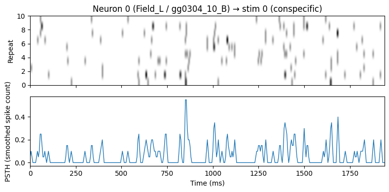
4. Visualizing a response

Responses are spike-count tensors per (stim, neuron) pair, shaped (R, T) — one row per repeat. The trial-averaged PSTH is response.mean(dim=0).

Note: missing (stim, neuron) pairs are (1, 1) NaN tensors, so we pick a (stim, neuron) pair that nrn_masks confirms as real data.

# find a (s, n) pair that has real data
valid_pairs = aa1.nrn_masks.nonzero()
stim_idx, neuron_idx = valid_pairs[0].tolist()

spikes = aa1.responses[stim_idx][neuron_idx]        # (R, T)
psth = spikes.mean(dim=0)                            # (T,)
time_ms = torch.arange(spikes.shape[-1]) * aa1.dt

nrn = aa1.nrn_meta[neuron_idx]
stim_m = aa1.stim_meta[stim_idx]

fig, (ax0, ax1) = plt.subplots(2, 1, figsize=(8, 4), sharex=True)
ax0.imshow(spikes.numpy(), aspect="auto", cmap="Greys",
           extent=[0, float(time_ms[-1]), 0, spikes.shape[0]])
ax0.set_ylabel("Repeat")
ax0.set_title(f"Neuron {neuron_idx} ({nrn['area']} / {nrn['cell_id']}) "
              f"→ stim {stim_idx} ({stim_m['type']})")
ax1.plot(time_ms, psth.numpy(), lw=1)
ax1.set_xlabel("Time (ms)")
ax1.set_ylabel("PSTH (smoothed spike count)")
plt.tight_layout()
plt.show()

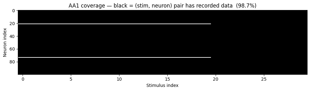
5. Coverage: the nrn_masks tensor

dataset.nrn_masks is a derived (S, N) bool tensor, True iff neuron n has real data for stimulus s. It is computed on the fly from the NaN sentinels — the single source of truth is self.responses. A heatmap exposes the sparse coverage pattern.

fig, ax = plt.subplots(figsize=(10, 3))
ax.imshow(aa1.nrn_masks.T.numpy(), aspect="auto", cmap="Greys", interpolation="nearest")
ax.set_xlabel("Stimulus index")
ax.set_ylabel("Neuron index")
ax.set_title(f"AA1 coverage — black = (stim, neuron) pair has recorded data  "
             f"({100 * aa1.nrn_masks.float().mean().item():.1f}%)")
plt.tight_layout()
plt.show()

6. Selecting a sub-population

__getitem__ and __len__ operate on the subset of neurons currently selected by self.I. Three helpers populate it:

• select_neuron(i) — single neuron by integer index.

• select_population([i, j, …]) — an explicit list of indices.

• select_pop_by_nrn_attr(attr, value) — all neurons whose nrn_meta[attr] == value. Dict-based metadata makes this idiomatic: e.g. select_pop_by_nrn_attr("area", "MLd").

Selection is stateful — call as many times as you like; the dataset reflects the most recent call on every subsequent __getitem__.

aa1.select_pop_by_nrn_attr("area", "MLd")

print(f"Selected {len(aa1.I)} MLd neurons out of {aa1.N_neurons} total.")
print(f"len(aa1) now returns: {len(aa1)}  (stims with >=1 valid selected neuron)")

Selected 50 MLd neurons out of 100 total.
len(aa1) now returns: 30  (stims with >=1 valid selected neuron)

6.1 What len(ds) and ds[i] actually expose

A subtle but important detail: both len(ds) and ds[i] are filtered by the current neuron selection. They expose only the stimuli for which at least one currently selected neuron has valid response data. Stimuli that the selection has no data on are hidden — len(ds) does not count them, and ds[i] never returns them.

This is what makes a DataLoader(ds, ...) safe under any selection: iterating range(len(ds)) is guaranteed to visit only stimuli with real response data for the selected neurons, never a fully-NaN slab.

The stored attributes (ds.stims, ds.responses, ds.stim_meta, ds.nrn_masks, …) are not filtered — they keep the dataset’s full structure regardless of self.I. Use them for direct access to a specific raw stim. The filter applies only at the iteration interface.

# concrete demo of the filter: pick one neuron with sparse coverage and
# observe how len(ds) and the iterable space adapt.
aa1.select_neuron(neuron_idx)
print(f"selected: {aa1.nrn_meta[neuron_idx]['cell_id']}")
print(f"  this neuron has data for {int(aa1.nrn_masks[:, neuron_idx].sum())} / {aa1.get_S()} stims")
print(f"  len(aa1)               = {len(aa1)}    # exactly the iterable subset")
print(f"  aa1[0] stim_meta       = {aa1[0][3]}    # first iterable stim")
try:
    aa1[len(aa1)]
except IndexError as e:
    print(f"  aa1[len(aa1)]          -> IndexError (no fully-NaN slab returned)")
print(f"  aa1.stims[0] is still raw stim 0 ({aa1.stim_meta[0]['type']}); "
      f"raw access bypasses the filter.")

selected: gg0304_10_B
  this neuron has data for 30 / 30 stims
  len(aa1)               = 30    # exactly the iterable subset
  aa1[0] stim_meta       = {'name': '058767E725C83836F405A97FD7D1E751.wav', 'type': 'conspecific'}    # first iterable stim
  aa1[len(aa1)]          -> IndexError (no fully-NaN slab returned)
  aa1.stims[0] is still raw stim 0 (conspecific); raw access bypasses the filter.

7. Batching with a DataLoader

Because stim duration T_s and repeat count R_{s,n} both vary across items, the default PyTorch collate cannot stack items into a single tensor. Use deepSTRF.utils.data.neural_collate, which right-pads stims with zeros and responses with NaN, then derives a valid_mask via ~responses.isnan().

One yielded batch is a 4-tuple: (stims, responses, valid_mask, stim_metas). See data_paradigm.md §5 for exact shapes and §6 for the recommended loss pattern (pred_psth[valid] boolean indexing).

loader = DataLoader(aa1, batch_size=4, shuffle=False, collate_fn=neural_collate)
batch = next(iter(loader))
stims, responses, valid_mask, stim_metas = batch['stims'], batch['responses'], batch['valid_mask'], batch['stim_meta']

print(f"stims shape       : {tuple(stims.shape)}       (B, 1, F, T_max)")
print(f"responses shape   : {tuple(responses.shape)}   (B, N_selected, R_max, T_max)")
print(f"valid_mask shape  : {tuple(valid_mask.shape)}  (B, N_selected, R_max, T_max) bool")
print(f"stim_metas        : {stim_metas}")
print()
print(f"valid fraction across the batch: {valid_mask.float().mean().item():.3f}")
print(f"per-item count of fully-NaN slabs (neuron×stim pairs without data): "
      f"{[int((~valid_mask[b].any(dim=(1, 2))).sum()) for b in range(valid_mask.shape[0])]}")

stims shape       : (4, 1, 32, 460)       (B, 1, F, T_max)
responses shape   : (4, 1, 10, 460)   (B, N_selected, R_max, T_max)
valid_mask shape  : (4, 1, 10, 460)  (B, N_selected, R_max, T_max) bool
stim_metas        : [{'name': '058767E725C83836F405A97FD7D1E751.wav', 'type': 'conspecific'}, {'name': '0A07B255BF830083B6726388CA8510BA.wav', 'type': 'conspecific'}, {'name': '1470489635DD93410408CE9F8FB2F7D9.wav', 'type': 'conspecific'}, {'name': '42FED9F3EF45A238202B050B06F91652.wav', 'type': 'conspecific'}]

valid fraction across the batch: 0.878
per-item count of fully-NaN slabs (neuron×stim pairs without data): [0, 0, 0, 0]

8. Switching to AA2

AA2 uses the exact same interface — just a different data directory and a richer set of recording areas and stimulus classes. Skipping the smoothing below to speed up instantiation.

aa2 = CRCNSAA2Dataset(
    download=True,
    areas=("Field_L", "mld", "OV", "CM"),
    stimuli=("conspecific", "songrip", "flatrip"),
    dt_ms=DT_MS,
    smooth=False,
)
print(aa2)
print(f"coverage: {int(aa2.nrn_masks.sum())} / {aa2.nrn_masks.numel()} "
      f"({100 * aa2.nrn_masks.float().mean().item():.1f}%)")
print(f"one nrn_meta entry: {aa2.nrn_meta[0]}")

# same API, same dict from the collate:
aa2.select_population(list(range(min(aa2.N_neurons, 32))))   # take 32 neurons to keep the batch small
loader = DataLoader(aa2, batch_size=4, shuffle=False, collate_fn=neural_collate)
batch = next(iter(loader))
stims, responses, valid_mask, stim_metas = batch['stims'], batch['responses'], batch['valid_mask'], batch['stim_meta']
print(f"AA2 batch stims shape      : {tuple(stims.shape)}")
print(f"AA2 batch responses shape  : {tuple(responses.shape)}")
print(f"AA2 batch valid_mask shape : {tuple(valid_mask.shape)}")

Recap

• Every deepSTRF dataset exposes the same core attributes — stims, responses, stim_meta, nrn_meta — plus the derived nrn_masks property, regardless of modality or source.

• Missingness on the response side is encoded as NaN (see data_paradigm.md §4 for why). The nrn_masks property is the canonical “does this (stim, neuron) pair have data” query — computed on the fly from responses.

• neural_collate handles the ragged batch-padding and emits a (B, N, R, T) valid_mask alongside the NaN-padded responses.

• Neuron sub-population selection is stateful via self.I — the same dataset object works as a single-neuron or a population dataset depending on the most recent select_* call.

Next: see the fit_audio_*.ipynb notebooks for examples of actually fitting a model on these datasets.