Learnable audio front-ends: beating the native spectrogram on NS1

deepSTRF can feed encoding models a raw waveform instead of a precomputed spectrogram: the model’s wav2spec slot turns audio into a neural-rate spectrogram, and — crucially — that transform can be learned. This notebook asks a concrete question:

Can a learnable front-end predict neurons better than the spectrogram the dataset authors shipped?

We compare two pipelines on NS1 (ferret A1), both with the same Linear STRF readout, changing only the front-end:

1. native spectrogram → Linear — the precomputed Rahman et al. (2019) cochleagram (X_nfht) that ships with NS1.

2. raw waveform → LEAF → Linear — a strictly-causal LEAF front-end (learnable Gabor filterbank + Gaussian pooling + per-channel PCEN) learned end-to-end with the readout.

Then we look at what LEAF learned — its filters and an example spectrogram — and close with an honest caveat about what the comparison does and does not show.

Setup — Google Colab

On Colab this installs deepSTRF from source; locally (pip install -e .) it is a no-op.

import sys
if 'google.colab' in sys.modules:
    !pip install -q git+https://github.com/urancon/deepSTRF.git
    print('deepSTRF installed from GitHub.')
else:
    print('Local environment — assuming deepSTRF is already importable.')

Local environment — assuming deepSTRF is already importable.

%matplotlib inline
import tempfile
import numpy as np
import torch
import matplotlib.pyplot as plt
from torch.utils.data import DataLoader, Subset

from deepSTRF.datasets.audio.ns1 import NS1Dataset
from deepSTRF.models.audio import Linear
from deepSTRF.models.wav2spec import CausalLEAF
from deepSTRF.training import Fitter
from deepSTRF.utils import neural_collate

DEVICE = 'cuda' if torch.cuda.is_available() else 'cpu'
print(f'Using device: {DEVICE}')

Using device: cuda

1. Load NS1 — spectrogram and waveform views

We instantiate the dataset twice. The responses are bit-identical between the two; only self.stims differs (precomputed (1, 34, 999) spectrogram vs (1, T_audio) waveform at audio_fs). The waveform is grid-locked to the response bins: T_audio = T_neural * ds.hop.

ds_spec = NS1Dataset(download=True)                       # precomputed X_nfht
ds_wav  = NS1Dataset(return_waveform=True, download=True) # raw waveform @ 48 kHz
N = ds_wav.N_neurons
print(f'N={N} cells | audio {ds_wav.audio_fs} Hz | hop={ds_wav.hop} samples/bin '
      f'| spec stim {tuple(ds_spec.stims[0].shape)} | wav stim {tuple(ds_wav.stims[0].shape)}')
print(f'ferret hearing range (informational): {ds_wav.hearing_range_hz} Hz')

N=119 cells | audio 48000 Hz | hop=240 samples/bin | spec stim (1, 34, 999) | wav stim (1, 239760)
ferret hearing range (informational): (200.0, 40000.0) Hz

2. Two pipelines, same readout

fit_and_report trains with early stopping (patience 30) and best-val checkpoint restoration (ckpt_path), so the reported test cc_norm is the best-validation model, not the final epoch. Same 14 / 3 / 3 stim split for both arms.

def fit_and_report(ds, model, label, *, lr=1e-3, max_epochs=100, patience=30):
    train = DataLoader(Subset(ds, range(14)),     batch_size=1, shuffle=True,  collate_fn=neural_collate)
    val   = DataLoader(Subset(ds, range(14, 17)), batch_size=1, shuffle=False, collate_fn=neural_collate)
    test  = DataLoader(Subset(ds, range(17, 20)), batch_size=1, shuffle=False, collate_fn=neural_collate)
    opt = torch.optim.AdamW(model.parameters(), lr=lr, weight_decay=0.0)
    ckpt = tempfile.NamedTemporaryFile(suffix='.pt', delete=False).name
    fitter = Fitter(model, train, val, optimizer=opt, device=DEVICE,
                    max_epochs=max_epochs, patience=patience,
                    monitor='val_cc_norm', mode='max', ckpt_path=ckpt,
                    log_fn=lambda d: None)
    fitter.fit()                                  # restores best-val weights
    cc = fitter.evaluate(test)['cc_norm'].cpu()
    n_params = sum(p.numel() for p in model.parameters() if p.requires_grad)
    return dict(label=label, cc=cc, mean=float(cc.mean()),
                median=float(cc.median()), n_params=n_params)

results = []

# Pipeline A — native precomputed spectrogram -> Linear
torch.manual_seed(0)
m_spec = Linear(n_frequency_bands=34, temporal_window_size=9, out_neurons=N)
results.append(fit_and_report(ds_spec, m_spec, 'native spec + Linear'))

# Pipeline B — raw waveform -> LEAF -> Linear (learned end-to-end)
torch.manual_seed(0)
m_leaf = Linear(n_frequency_bands=34, temporal_window_size=9, out_neurons=N,
                wav2spec=CausalLEAF(audio_fs=ds_wav.audio_fs, n_filters=34,
                                    hop_ms=ds_wav.dt, f_min=60.0, f_max=22627.0))
results.append(fit_and_report(ds_wav, m_leaf, 'waveform + LEAF + Linear', lr=3e-3))

for r in results:
    print(f"{r['label']:28s}  mean cc_norm = {r['mean']:.3f}  "
          f"median = {r['median']:.3f}  params = {r['n_params']:,}")

native spec + Linear          mean cc_norm = 0.552  median = 0.568  params = 36,771
waveform + LEAF + Linear      mean cc_norm = 0.708  median = 0.732  params = 37,009

3. What did LEAF learn? — the filters

LEAF’s Gabor filterbank starts mel-spaced (like the native cochleagram) but its centre frequencies are learnable. Unlike SincNet (whose cutoffs barely move), LEAF’s centres drift noticeably during training — the model retunes the filterbank to the neural data.

def gabor_center_hz(leaf):
    return (leaf.center_freq_.detach().cpu() * leaf.audio_fs / (2 * np.pi)).numpy()

leaf_trained = m_leaf.wav2spec
torch.manual_seed(0)
leaf_init = CausalLEAF(audio_fs=ds_wav.audio_fs, n_filters=34, hop_ms=ds_wav.dt,
                       f_min=60.0, f_max=22627.0)
fc_init, fc_trained = gabor_center_hz(leaf_init), gabor_center_hz(leaf_trained)

fig, axes = plt.subplots(1, 2, figsize=(12, 4))
idx = np.arange(len(fc_init))
axes[0].plot(idx, fc_init, 'o--', ms=3, label='init (mel-spaced)')
axes[0].plot(idx, fc_trained, 'x-', ms=4, label='learned')
axes[0].set_yscale('log'); axes[0].set_xlabel('filter index')
axes[0].set_ylabel('Gabor centre frequency (Hz)')
axes[0].set_title('LEAF centres: init vs learned'); axes[0].legend(); axes[0].grid(True, which='both', alpha=0.3)

# frequency responses of a few learned Gabor filters
real, imag = leaf_trained._build_gabor()
real = real.detach().cpu().squeeze(1).numpy()      # (F, K)
for k in (3, 11, 19, 27, 33):
    H = np.abs(np.fft.rfft(real[k], n=4096))
    freqs = np.fft.rfftfreq(4096, d=1.0 / leaf_trained.audio_fs) / 1000
    axes[1].plot(freqs, H / H.max(), lw=1.3, label=f'ch {k} ({fc_trained[k]:.0f} Hz)')
axes[1].set_xscale('log'); axes[1].set_xlim(0.05, 24)
axes[1].set_xlabel('frequency (kHz)'); axes[1].set_ylabel('|H(f)| (norm.)')
axes[1].set_title('learned Gabor filter responses'); axes[1].legend(fontsize=8); axes[1].grid(True, which='both', alpha=0.3)
plt.tight_layout(); plt.show()

drift = np.abs(fc_trained - fc_init) / fc_init
print(f'mean relative drift of Gabor centres: {drift.mean():.1%} '
      f'(vs SincNet, whose cutoffs move < 0.01%)')

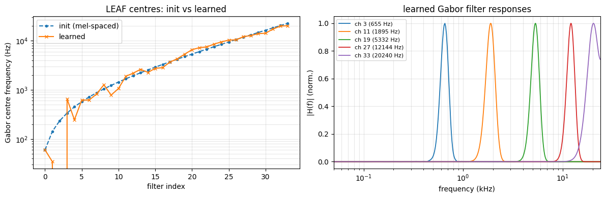
mean relative drift of Gabor centres: 20.1% (vs SincNet, whose cutoffs move < 0.01%)

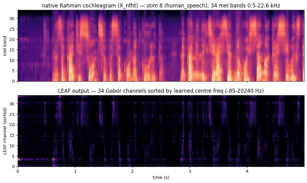
4. The learned spectrogram vs the native one

Below: the same stimulus through LEAF and through the native Rahman cochleagram.

Mind the frequency axis. The two front-ends do not share a frequency ladder: the native X_nfht is fixed mel-spaced (500–22 627 Hz, Rahman/voicebox convention), while LEAF’s 34 channels sit at their learned centre frequencies. We therefore sort the LEAF channels by learned centre frequency and label both axes with their own Hz range — they are not bin-for-bin comparable, only qualitatively.

stim_idx = 8
with torch.no_grad():
    leaf_out = leaf_trained(ds_wav.stims[stim_idx].unsqueeze(0).to(DEVICE)).squeeze().cpu().numpy()
native = ds_spec.stims[stim_idx].squeeze().numpy()
order = np.argsort(fc_trained)                      # sort LEAF channels low->high Hz
fc_sorted = fc_trained[order]

fig, axs = plt.subplots(2, 1, figsize=(10, 6), sharex=True)
axs[0].imshow(native, aspect='auto', origin='lower', cmap='magma',
              extent=(0, 4.995, 0, 34))
axs[0].set_title(f'native Rahman cochleagram (X_nfht) — stim {stim_idx} '
                 f'({ds_spec.stim_meta[stim_idx]["type"]}); 34 mel bands 0.5-22.6 kHz')
axs[0].set_ylabel('mel band')
axs[1].imshow(leaf_out[order], aspect='auto', origin='lower', cmap='magma',
              extent=(0, 4.995, 0, 34))
axs[1].set_title(f'LEAF output — 34 Gabor channels sorted by learned centre freq '
                 f'({fc_sorted[0]:.0f}-{fc_sorted[-1]:.0f} Hz)')
axs[1].set_ylabel('LEAF channel (sorted)'); axs[1].set_xlabel('time (s)')
plt.tight_layout(); plt.show()

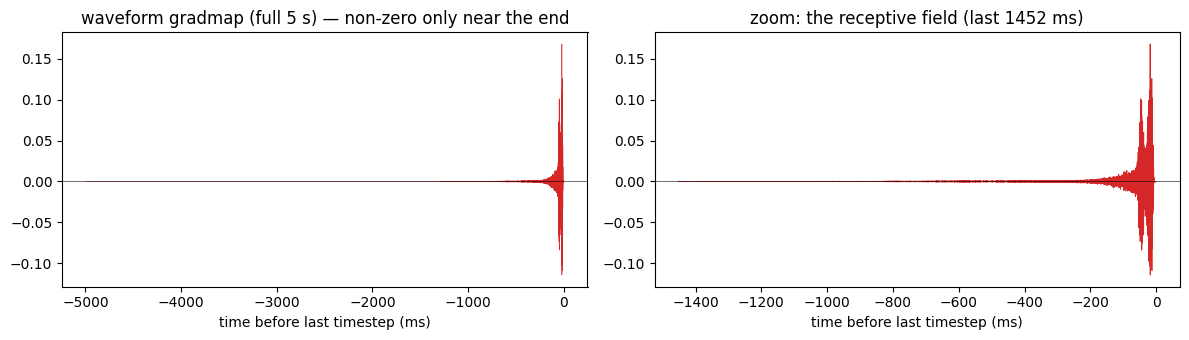
5. The waveform receptive field — see it and hear it

Because the front-end is part of the model, we can backprop a neuron’s response all the way to the raw audio samples — model.waveform_gradmap(...). The result is itself a waveform: a time-domain receptive field (RF), only possible with a wav-native model.

By default (reduce='last', matching STRF_gradmap) we maximize the activation at the last timestep, so the gradient is supported only within the RF window before that timestep and decays to ~zero further into the past — by causality and the finite STRF. (Using reduce='sum' instead would integrate over all 999 output timesteps and be non-zero over the whole 5 s — a whole-stimulus saliency map, not an RF.) Watch how short the RF is:

from IPython.display import Audio, display

stim = ds_wav.stims[stim_idx].to(DEVICE)                 # (1, T_audio)
with torch.no_grad():
    pred = m_leaf(stim.unsqueeze(0))[0, :, 0, :]         # (N, T_neural)
best_neuron = int(pred.max(dim=1).values.argmax())      # most strongly driven cell

gradmap = m_leaf.waveform_gradmap(stim, neuron=best_neuron).cpu().numpy()  # reduce='last'
t_ms = (np.arange(len(gradmap)) - len(gradmap) + 1) / ds_wav.audio_fs * 1000  # ms before last sample

# where does 99% of the RF mass sit (measured back from the end)?
mass = np.cumsum(np.abs(gradmap)[::-1])
rf_ms = np.searchsorted(mass, 0.99 * mass[-1]) / ds_wav.audio_fs * 1000
print(f'cell #{best_neuron}: 99% of the RF gradient mass is within the last {rf_ms:.0f} ms '
      f'(bare STRF window = {9 * ds_wav.dt:.0f} ms; the extra reach is LEAF/PCEN memory)')

win_s = float(min(2.0, max(0.3, 1.3 * rf_ms / 1000)))   # cover the RF, capped at 2 s
zoom = int(win_s * ds_wav.audio_fs)
fig, ax = plt.subplots(1, 2, figsize=(12, 3.5))
ax[0].plot(t_ms, gradmap, lw=0.4, color='C3')
ax[0].set_title('waveform gradmap (full 5 s) — non-zero only near the end')
ax[1].plot(t_ms[-zoom:], gradmap[-zoom:], lw=0.6, color='C3')
ax[1].set_title(f'zoom: the receptive field (last {win_s*1000:.0f} ms)')
for a in ax:
    a.set_xlabel('time before last timestep (ms)'); a.axhline(0, color='k', lw=0.4)
plt.tight_layout(); plt.show()

cell #3: 99% of the RF gradient mass is within the last 1117 ms (bare STRF window = 45 ms; the extra reach is LEAF/PCEN memory)

def _norm(w):
    w = np.asarray(w, dtype=np.float32)
    return w / (np.abs(w).max() + 1e-9)

# crop both to the RF window so the clips are short.
rf_audio  = gradmap[-zoom:]
stim_rf   = ds_wav.stims[stim_idx].squeeze().numpy()[-zoom:]

# Playable audio widgets bloat the committed notebook, so the docs ship without
# them. Set EMBED_AUDIO = True (or just run this cell yourself) to listen.
EMBED_AUDIO = False
if EMBED_AUDIO:
    print(f'Last {win_s*1000:.0f} ms of the stimulus (what the cell heard in its RF window):')
    display(Audio(_norm(stim_rf), rate=ds_wav.audio_fs))
    print(f"Cell #{best_neuron}'s receptive field (gradmap) — listen to what drives it:")
    display(Audio(_norm(rf_audio), rate=ds_wav.audio_fs))

Takeaways

• A learned front-end can beat the dataset’s native spectrogram. On NS1, waveform → LEAF → Linear predicts cortical responses substantially better than native spec → Linear — and LEAF’s filterbank visibly retunes itself to the data (its Gabor centres drift, unlike SincNet’s frozen cutoffs).

• Honest caveat — this is more than a front-end swap. LEAF adds real learnable feature extraction (~6 parameters per channel: Gabor frequency + bandwidth, pooling width, and per-channel learnable PCEN), so LEAF + Linear is effectively a shallow nonlinear model, not just a different spectrogram feeding the same model. The fair reading is “a learnable front-end lets a thin readout punch above its weight,” not “LEAF’s spectrogram is intrinsically better than mel.”

• It depends on the downstream model. With an expressive model (StateNet), the picture inverts: a clean fixed mel front-end is best, the learnable front-ends roughly tie it, and adaptive compression (PCEN) can even hurt — the RNN already does the representational work a Linear readout cannot. Front-end learnability helps inversely with model capacity.

• Waveform-native models are interpretable in the audio domain. Because the spectrogram transform is inside the model, waveform_gradmap (default reduce='last', maximizing the last timestep like STRF_gradmap) gives each neuron a time-domain receptive field you can plot and listen to — something a fixed-spectrogram pipeline cannot do. The RF is localized (the gradient vanishes beyond it, by causality + the finite STRF), but note LEAF’s PCEN gain-control learned a fairly long temporal memory here (hundreds of ms, vs the 45 ms bare STRF) — flexible, though likely longer than a biological A1 RF, consistent with the added-capacity caveat above.

See `wav2spec.md <../docs/_source/md/wav2spec.md>`__ for the front-end zoo and the strict-causality contract, and `fit_ns1_linear_from_waveform.ipynb <fit_ns1_linear_from_waveform.ipynb>`__ for the mel / SincNet / ICNet walk-through.