Fitting NS1 auditory cortical responses with StateNet

This notebook is the canonical end-to-end demo of deepSTRF: dataset → model → metrics → training. It uses the NS1 dataset (Harper et al. 2016, Rahman et al. 2020; auto-downloaded from OSF + the DNet companion repo) and a StateNet GRU encoding model (Rahman, Willmore et al. 2020), trained with the deepSTRF `Fitter <../docs/_source/md/fitter.md>`__.

What you’ll see:

1. Auto-download and inspect NS1 (119 ferret A1 cells, 20 nat. sound clips, R=20 reps).

2. Train/val/test split by stimulus (14 / 3 / 3).

3. Build a StateNet GRU population model (one model fits all 119 cells jointly).

4. Train with the Fitter, monitoring val_cc_norm (Schoppe-style noise-corrected correlation; see `metrics_paradigm.md <../docs/_source/md/metrics_paradigm.md>`__ §6.4).

5. Evaluate on the held-out test stimuli and visualise predictions vs PSTHs.

Reference numbers for orientation: published mean cc_norm for StateNet on NS1 is ~0.7–0.8 with leave-one-out training; this minimal 14-stim train set lands in the same neighbourhood.

Setup — Google Colab

If you’re running on Google Colab, the cell below installs deepSTRF from source. On a local install (pip install -e .) it’s a no-op.

import sys
if 'google.colab' in sys.modules:
    !pip install -q git+https://github.com/urancon/deepSTRF.git
    print("deepSTRF installed from GitHub.")
else:
    print("Local environment — assuming deepSTRF is already importable.")

Imports

%matplotlib inline
import matplotlib.pyplot as plt
import numpy as np
import torch
import torch.nn as nn
from torch.utils.data import DataLoader, Subset

from deepSTRF.datasets.audio.ns1 import NS1Dataset
from deepSTRF.models.audio import StateNet
from deepSTRF.metrics import corrcoef, normalized_corrcoef
from deepSTRF.training import Fitter, set_random_seed
from deepSTRF.utils import neural_collate, plot_stim_with_response, plot_psth_vs_pred

device = "cuda" if torch.cuda.is_available() else "cpu"
print(f"Using device: {device}")
set_random_seed(0)

Using device: cuda

1. Load NS1

NS1Dataset(download=True) fetches metadata, raw spike data, and the precomputed 5 ms mel-spectrogram from public OSF + GitHub repos (~160 MB, no account needed). Subsequent loads use the cached copy under ~/.cache/deepSTRF/NS1.

ds = NS1Dataset(dt_ms=5.0, smooth=True, download=True)
print(f"Cells:      {ds.N_neurons}")
print(f"Stimuli:    {len(ds.stims)}")
print(f"Spec shape: {tuple(ds.stims[0].shape)}  (1, F, T) at dt=5 ms")
print(f"Resp shape: {tuple(ds.responses[0][0].shape)}  (R, T) per (stim, neuron)")
print(f"Stim types: {sorted(set(m['type'] for m in ds.stim_meta))}")

Cells:      119
Stimuli:    20
Spec shape: (1, 34, 999)  (1, F, T) at dt=5 ms
Resp shape: (20, 999)  (R, T) per (stim, neuron)
Stim types: ['ferret_vocalization', 'human_speech', 'insects_buzzing', 'unknown', 'water_sounds']

2. Quick look — one stim, one cell

The stimulus is a 4.995-s 34-band mel spectrogram. The response is 20 trial repeats binned at 5 ms, smoothed with a 21 ms Hanning window (Hsu, Borst & Theunissen 2004 convention).

stim_idx, cell_idx = 0, 5
spec = ds.stims[stim_idx]                          # (1, F, T)
resp = ds.responses[stim_idx][cell_idx]            # (R, T)

plot_stim_with_response(
    spec, resp, dt_ms=5,
    title=(f"NS1 stim {stim_idx} — '{ds.stim_meta[stim_idx]['name']}' "
           f"({ds.stim_meta[stim_idx]['type']}) → cell {cell_idx}"),
)
plt.show()

psth = resp.mean(dim=0).numpy()
print(f"PSTH range: [{psth.min():.3f}, {psth.max():.3f}]  mean: {psth.mean():.3f}")

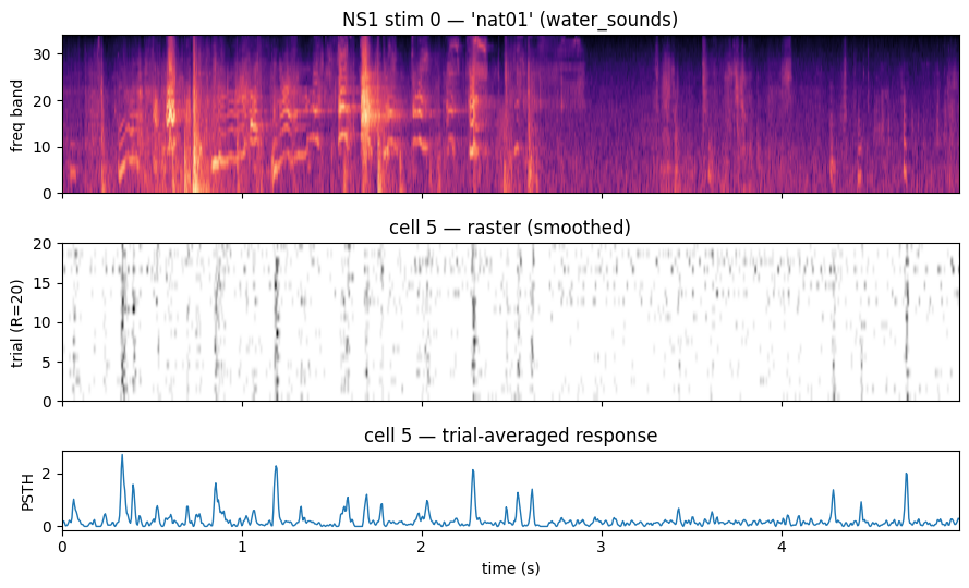
PSTH range: [0.000, 2.700]  mean: 0.224

3. Train / val / test split

For this minimal demo we hold out 3 stims for validation and 3 for test. The published NS1 protocol uses leave-one-out cross-validation across all 20 stims; the same Fitter-based code generalises to that with an outer loop over splits.

train_idx = list(range(14))           # stims 0..13
val_idx   = list(range(14, 17))       # 14, 15, 16
test_idx  = list(range(17, 20))       # 17, 18, 19

train_loader = DataLoader(Subset(ds, train_idx), batch_size=1,
                          shuffle=True, collate_fn=neural_collate)
val_loader   = DataLoader(Subset(ds, val_idx),   batch_size=1,
                          shuffle=False, collate_fn=neural_collate)
test_loader  = DataLoader(Subset(ds, test_idx),  batch_size=1,
                          shuffle=False, collate_fn=neural_collate)

print(f"train: {len(train_loader.dataset)} stims | "
      f"val: {len(val_loader.dataset)} | "
      f"test: {len(test_loader.dataset)}")

train: 14 stims | val: 3 | test: 3

4. Model: StateNet GRU

StateNet (Rahman, Willmore et al. 2020) is a per-timestep spectral encoder followed by a recurrent core (GRU here) and a per-neuron linear readout. With out_neurons=119, one population model jointly fits all NS1 cells through a shared backbone.

The default output activation is ParametricSoftplus(out_neurons) — per-neuron learnable sharpness β and additive baseline b, both softplus-reparameterised so the curve stays non-negative. This is unbounded above (good for spike-count regression where peaks can exceed

1. and the per-neuron parameters let the model adapt the firing curve per cell. See deepSTRF.models.activations for the alternative parametric variants (ParametricSigmoid, ParametricDoubleExponential) or pass output_activation=nn.Identity() for an unbounded signed output.

model = StateNet(
    n_frequency_bands=34,
    hidden_channels=7, kernel_size=7, stride=3,
    connectivity="LC", rnn_type="GRU",
    out_neurons=ds.N_neurons,
)
print(model)
print(f"\nTrainable params: {model.count_trainable_params():,}")

StateNet(
  (wav2spec): Identity()
  (prefiltering): Identity()
  (core): Identity()
  (encoder_layers): Sequential(
    (0): LocallyConnected1d(
      (unfold): Unfold(kernel_size=(7, 1), dilation=1, padding=0, stride=3)
      (fold): Fold(output_size=(10, 1), kernel_size=(1, 1), dilation=1, padding=0, stride=1)
    )
    (1): CausalLayerNorm(
      (ln): LayerNorm((7,), eps=1e-05, elementwise_affine=True)
    )
    (2): Sigmoid()
  )
  (rnn): GRU(70, 70, batch_first=True)
  (readout): LinearReadout(
    (fc): Linear(in_features=70, out_features=119, bias=True)
    (activation): ParametricSoftplus(N=119, non_negative_output=True)
  )
)

Trainable params: 39,081

5. Train with the Fitter

The Fitter wires a model, the loaders, an optimizer, and the canonical val metrics (cc, cc_norm) into a single .fit() call. Defaults match metrics_paradigm.md §7: mse_loss against the auto-PSTH of responses, monitor='val_cc_norm' with mode='max', and AdamW with lr=1e-3. We override weight_decay=0.0 to match the legacy NS1 convention.

optimizer = torch.optim.AdamW(model.parameters(), lr=1e-3, weight_decay=0.0)

fitter = Fitter(
    model, train_loader, val_loader,
    optimizer=optimizer,
    device=device,
    max_epochs=80,
    patience=15,
    monitor="val_cc_norm",
    mode="max",
    log_fn=lambda d: print(
        f"epoch {d['epoch']:3d}  "
        f"train_loss={d['train_loss']:.4f}  "
        f"val_loss={d['val_loss']:.4f}  "
        f"val_cc_norm={torch.nanmean(d['val_cc_norm']):+.3f}",
        flush=True,
    ),
)
history = fitter.fit()
print(f"\nfinished after {len(history)} epochs")

epoch   0  train_loss=0.0305  val_loss=0.0204  val_cc_norm=+0.112
epoch   1  train_loss=0.0244  val_loss=0.0192  val_cc_norm=+0.161
epoch   2  train_loss=0.0236  val_loss=0.0189  val_cc_norm=+0.204
epoch   3  train_loss=0.0230  val_loss=0.0185  val_cc_norm=+0.250
epoch   4  train_loss=0.0224  val_loss=0.0185  val_cc_norm=+0.293
epoch   5  train_loss=0.0222  val_loss=0.0180  val_cc_norm=+0.338
epoch   6  train_loss=0.0218  val_loss=0.0175  val_cc_norm=+0.381
epoch   7  train_loss=0.0212  val_loss=0.0171  val_cc_norm=+0.418
epoch   8  train_loss=0.0204  val_loss=0.0168  val_cc_norm=+0.471
epoch   9  train_loss=0.0197  val_loss=0.0158  val_cc_norm=+0.517
epoch  10  train_loss=0.0191  val_loss=0.0154  val_cc_norm=+0.542
epoch  11  train_loss=0.0188  val_loss=0.0155  val_cc_norm=+0.561
epoch  12  train_loss=0.0184  val_loss=0.0151  val_cc_norm=+0.581
epoch  13  train_loss=0.0177  val_loss=0.0148  val_cc_norm=+0.599
epoch  14  train_loss=0.0175  val_loss=0.0150  val_cc_norm=+0.608
epoch  15  train_loss=0.0171  val_loss=0.0142  val_cc_norm=+0.631
epoch  16  train_loss=0.0165  val_loss=0.0141  val_cc_norm=+0.641
epoch  17  train_loss=0.0162  val_loss=0.0139  val_cc_norm=+0.656
epoch  18  train_loss=0.0161  val_loss=0.0136  val_cc_norm=+0.666
epoch  19  train_loss=0.0156  val_loss=0.0138  val_cc_norm=+0.672
epoch  20  train_loss=0.0157  val_loss=0.0140  val_cc_norm=+0.680
epoch  21  train_loss=0.0156  val_loss=0.0133  val_cc_norm=+0.694
epoch  22  train_loss=0.0154  val_loss=0.0142  val_cc_norm=+0.698
epoch  23  train_loss=0.0157  val_loss=0.0129  val_cc_norm=+0.706
epoch  24  train_loss=0.0151  val_loss=0.0135  val_cc_norm=+0.703
epoch  25  train_loss=0.0149  val_loss=0.0130  val_cc_norm=+0.712
epoch  26  train_loss=0.0145  val_loss=0.0127  val_cc_norm=+0.721
epoch  27  train_loss=0.0144  val_loss=0.0126  val_cc_norm=+0.726
epoch  28  train_loss=0.0143  val_loss=0.0122  val_cc_norm=+0.736
epoch  29  train_loss=0.0141  val_loss=0.0122  val_cc_norm=+0.738
epoch  30  train_loss=0.0139  val_loss=0.0123  val_cc_norm=+0.739
epoch  31  train_loss=0.0139  val_loss=0.0124  val_cc_norm=+0.738
epoch  32  train_loss=0.0137  val_loss=0.0119  val_cc_norm=+0.752
epoch  33  train_loss=0.0137  val_loss=0.0119  val_cc_norm=+0.757
epoch  34  train_loss=0.0135  val_loss=0.0118  val_cc_norm=+0.758
epoch  35  train_loss=0.0134  val_loss=0.0117  val_cc_norm=+0.764
epoch  36  train_loss=0.0133  val_loss=0.0117  val_cc_norm=+0.766
epoch  37  train_loss=0.0132  val_loss=0.0116  val_cc_norm=+0.765
epoch  38  train_loss=0.0131  val_loss=0.0115  val_cc_norm=+0.773
epoch  39  train_loss=0.0131  val_loss=0.0115  val_cc_norm=+0.775
epoch  40  train_loss=0.0130  val_loss=0.0115  val_cc_norm=+0.772
epoch  41  train_loss=0.0129  val_loss=0.0114  val_cc_norm=+0.779
epoch  42  train_loss=0.0128  val_loss=0.0115  val_cc_norm=+0.780
epoch  43  train_loss=0.0128  val_loss=0.0114  val_cc_norm=+0.781
epoch  44  train_loss=0.0127  val_loss=0.0113  val_cc_norm=+0.783
epoch  45  train_loss=0.0127  val_loss=0.0113  val_cc_norm=+0.785
epoch  46  train_loss=0.0126  val_loss=0.0113  val_cc_norm=+0.788
epoch  47  train_loss=0.0127  val_loss=0.0114  val_cc_norm=+0.780
epoch  48  train_loss=0.0127  val_loss=0.0116  val_cc_norm=+0.783
epoch  49  train_loss=0.0126  val_loss=0.0112  val_cc_norm=+0.794
epoch  50  train_loss=0.0124  val_loss=0.0113  val_cc_norm=+0.791
epoch  51  train_loss=0.0123  val_loss=0.0112  val_cc_norm=+0.795
epoch  52  train_loss=0.0123  val_loss=0.0110  val_cc_norm=+0.800
epoch  53  train_loss=0.0123  val_loss=0.0112  val_cc_norm=+0.797
epoch  54  train_loss=0.0123  val_loss=0.0113  val_cc_norm=+0.786
epoch  55  train_loss=0.0123  val_loss=0.0111  val_cc_norm=+0.799
epoch  56  train_loss=0.0122  val_loss=0.0111  val_cc_norm=+0.800
epoch  57  train_loss=0.0120  val_loss=0.0111  val_cc_norm=+0.798
epoch  58  train_loss=0.0121  val_loss=0.0110  val_cc_norm=+0.799
epoch  59  train_loss=0.0120  val_loss=0.0111  val_cc_norm=+0.798
epoch  60  train_loss=0.0119  val_loss=0.0109  val_cc_norm=+0.804
epoch  61  train_loss=0.0119  val_loss=0.0111  val_cc_norm=+0.799
epoch  62  train_loss=0.0118  val_loss=0.0110  val_cc_norm=+0.803
epoch  63  train_loss=0.0118  val_loss=0.0113  val_cc_norm=+0.791
epoch  64  train_loss=0.0117  val_loss=0.0109  val_cc_norm=+0.806
epoch  65  train_loss=0.0117  val_loss=0.0109  val_cc_norm=+0.806
epoch  66  train_loss=0.0118  val_loss=0.0111  val_cc_norm=+0.808
epoch  67  train_loss=0.0117  val_loss=0.0109  val_cc_norm=+0.805
epoch  68  train_loss=0.0118  val_loss=0.0109  val_cc_norm=+0.808
epoch  69  train_loss=0.0117  val_loss=0.0107  val_cc_norm=+0.813
epoch  70  train_loss=0.0115  val_loss=0.0109  val_cc_norm=+0.807
epoch  71  train_loss=0.0115  val_loss=0.0109  val_cc_norm=+0.809
epoch  72  train_loss=0.0115  val_loss=0.0108  val_cc_norm=+0.813
epoch  73  train_loss=0.0114  val_loss=0.0108  val_cc_norm=+0.812
epoch  74  train_loss=0.0114  val_loss=0.0110  val_cc_norm=+0.801
epoch  75  train_loss=0.0114  val_loss=0.0110  val_cc_norm=+0.805
epoch  76  train_loss=0.0114  val_loss=0.0110  val_cc_norm=+0.804
epoch  77  train_loss=0.0112  val_loss=0.0108  val_cc_norm=+0.810
epoch  78  train_loss=0.0112  val_loss=0.0107  val_cc_norm=+0.811
epoch  79  train_loss=0.0112  val_loss=0.0108  val_cc_norm=+0.811

finished after 80 epochs

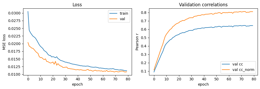
6. Training curves

epochs = [h["epoch"] for h in history]
train_loss = [h["train_loss"] for h in history]
val_loss = [h["val_loss"] for h in history]
val_cc = [torch.nanmean(h["val_cc"]).item() for h in history]
val_ccn = [torch.nanmean(h["val_cc_norm"]).item() for h in history]

fig, axs = plt.subplots(1, 2, figsize=(10, 3.5))
axs[0].plot(epochs, train_loss, label="train", lw=1.5)
axs[0].plot(epochs, val_loss, label="val", lw=1.5)
axs[0].set_xlabel("epoch"); axs[0].set_ylabel("MSE loss"); axs[0].legend()
axs[0].set_title("Loss")

axs[1].plot(epochs, val_cc, label="val cc",       lw=1.5)
axs[1].plot(epochs, val_ccn, label="val cc_norm", lw=1.5)
axs[1].set_xlabel("epoch"); axs[1].set_ylabel("Pearson r"); axs[1].legend()
axs[1].set_title("Validation correlations")
plt.tight_layout(); plt.show()

7. Test-set evaluation

fitter.evaluate(loader) runs the same cross-batch concat-then-compute pipeline on the held-out stims and returns un-prefixed metrics.

test_metrics = fitter.evaluate(test_loader)
test_cc = test_metrics["cc"].cpu()
test_ccn = test_metrics["cc_norm"].cpu()
print(f"test loss:       {test_metrics['loss']:.4f}")
print(f"test cc      mean={torch.nanmean(test_cc):+.3f}  median={torch.nanmedian(test_cc):+.3f}")
print(f"test cc_norm mean={torch.nanmean(test_ccn):+.3f}  median={torch.nanmedian(test_ccn):+.3f}")

test loss:       0.0160
test cc      mean=+0.659  median=+0.681
test cc_norm mean=+0.770  median=+0.796

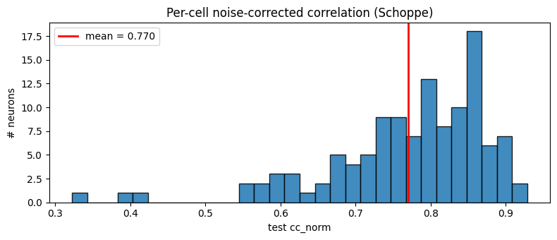
8. Per-cell cc_norm distribution

fig, ax = plt.subplots(figsize=(8, 3.5))
ax.hist(test_ccn.numpy(), bins=30, edgecolor="black", alpha=0.85)
ax.axvline(torch.nanmean(test_ccn).item(), color="red", lw=2,
           label=f"mean = {torch.nanmean(test_ccn):.3f}")
ax.set_xlabel("test cc_norm")
ax.set_ylabel("# neurons")
ax.set_title("Per-cell noise-corrected correlation (Schoppe)")
ax.legend()
plt.tight_layout(); plt.show()

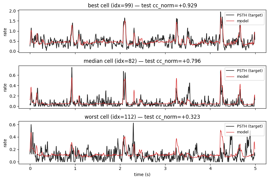
9. Predictions vs ground-truth PSTH

Pick the best, median, and worst cells (by test cc_norm) and overlay the model’s prediction on the trial-averaged response for one held-out stimulus.

# rank cells by cc_norm; pick best / median / worst
ranking = test_ccn.argsort(descending=True)
best, median, worst = ranking[0].item(), ranking[len(ranking) // 2].item(), ranking[-1].item()
picks = [("best", best), ("median", median), ("worst", worst)]

# run inference on test stim 0
model.eval()
with torch.no_grad():
    stim0 = ds.stims[test_idx[0]].unsqueeze(0).to(device)        # (1, 1, F, T)
    pred  = model(stim0).cpu().squeeze(0).squeeze(1)             # (N, T)

# trial-averaged response per cell on the same stim
psth_per_cell = torch.stack([r.mean(dim=0) for r in ds.responses[test_idx[0]]])  # (N, T)

fig, axs = plt.subplots(3, 1, figsize=(9, 6), sharex=True)
for ax, (label, idx) in zip(axs, picks):
    plot_psth_vs_pred(
        psth_per_cell[idx], pred[idx], dt_ms=5, ax=ax,
        title=f"{label} cell (idx={idx}) — test cc_norm={test_ccn[idx]:+.3f}",
    )
axs[-1].set_xlabel("time (s)")
plt.tight_layout(); plt.show()

What’s next

• Other audio datasets — same Fitter/metrics stack works on CRCNS AA1/AA2/AA4 and NAT4 with no code changes; only the dataset constructor differs.

• Cross-species concatenation — concat_neural_datasets([ns1, aa1]) builds a block-diagonal joint dataset; a single StateNet over the union fits both species jointly. See `dataset_concatenation.md <../docs/_source/md/dataset_concatenation.md>`__.

• Custom training loops — the Fitter is a thin convenience; for multi-GPU, mixed-precision, gradient accumulation, etc., write the 3-line canonical loop from `metrics_paradigm.md <../docs/_source/md/metrics_paradigm.md>`__ §7 directly.