Exploring NAT4 — the deepSTRF data paradigm in action

This notebook walks through the NAT4 dataset (Pennington & David 2023; auto-downloaded from Zenodo) as a hands-on tour of the deepSTRF data API. NAT4 is the dataset that exercises every subtle bit of the `data_paradigm.md <../docs/_source/md/data_paradigm.md>`__:

• Sparse coverage — not every cell saw every stimulus (33 of 849 A1 cells have no validation data); missing pairs are NaN-padded sentinels.

• Estimation / validation split — 575 est + 18 val stims, with a stim_meta['subset'] tag and a subset='all'|'est'|'val' constructor shortcut.

• Per-cell metadata richness — cell IDs parsed into site / animal / electrode / unit-in-electrode + auditory / depth tags.

• The bidirectional rule — selecting a stim subset auto-hides neurons whose only valid responses lie outside that subset.

• ``valid_mask`` — the bool grid the dataloader emits alongside responses, derived from NaN sentinels at collate time.

We focus on A1 here; the notebook closes with a brief PEG comparison and a cross-area concatenation example.

Setup — Google Colab

If you’re running on Google Colab, the cell below installs deepSTRF from source. On a local install (pip install -e .) it’s a no-op.

import sys
if 'google.colab' in sys.modules:
    !pip install -q git+https://github.com/urancon/deepSTRF.git
    print("deepSTRF installed from GitHub.")
else:
    print("Local environment — assuming deepSTRF is already importable.")

Imports

%matplotlib inline
import matplotlib.pyplot as plt
import numpy as np
import torch
from collections import Counter
from torch.utils.data import DataLoader, Subset

from deepSTRF.datasets.audio.nat4 import NAT4Dataset
from deepSTRF.utils import (
    neural_collate, concat_neural_datasets, plot_stim_with_response,
)

1. Load NAT4 A1

NAT4Dataset(area='A1', download=True) fetches 3 archives from Zenodo (~30 MB main + ~70 MB single-sites + 70 kB CSV) and unpacks them under ~/.cache/deepSTRF/NAT4/A1/. Subsequent loads use the cache. The default subset='all' loads both estimation and validation stims; for training-only workflows, subset='est' loads only the 575 estimation stims (faster).

ds = NAT4Dataset(area='A1', download=True, subset='all')
print(f"Cells:    {ds.N_neurons}")
print(f"Stimuli:  {len(ds.stims)}")
counts = Counter(m['subset'] for m in ds.stim_meta)
print(f"  est:    {counts['est']}")
print(f"  val:    {counts['val']}")
print(f"Spec shape: {tuple(ds.stims[0].shape)}  (1, F, T) at dt={ds.dt} ms")

NAT4 A1 val sites: 100%|██████████| 22/22 [00:08<00:00,  2.50it/s]

Cells:    849
Stimuli:  593
  est:    575
  val:    18
Spec shape: (1, 18, 150)  (1, F, T) at dt=10.0 ms

2. Per-cell metadata

Every neuron carries a metadata dict with the cell ID parsed into its recording site, animal (3-letter prefix), electrode, and unit-in-electrode. NAT4 also marks the auditory-vs-non-auditory classification used by Pennington & David (2023).

print("First 3 entries:")
for n in ds.nrn_meta[:3]:
    print(f"  {n}")
print()
n_auditory = sum(1 for n in ds.nrn_meta if n['auditory'])
print(f"auditory cells: {n_auditory} / {ds.N_neurons}")
animals = Counter(n['animal'] for n in ds.nrn_meta)
print(f"animals:        {dict(animals)}")
sites = Counter(n['site'] for n in ds.nrn_meta)
print(f"recording sites: {len(sites)} unique  (top 5: {sites.most_common(5)})")

First 3 entries:
  {'cell_id': 'ARM029a-04-1', 'area': 'A1', 'auditory': True, 'site': 'ARM029a', 'animal': 'ARM', 'electrode': 4, 'unit_in_electrode': 1}
  {'cell_id': 'ARM029a-07-6', 'area': 'A1', 'auditory': True, 'site': 'ARM029a', 'animal': 'ARM', 'electrode': 7, 'unit_in_electrode': 6}
  {'cell_id': 'ARM029a-07-7', 'area': 'A1', 'auditory': True, 'site': 'ARM029a', 'animal': 'ARM', 'electrode': 7, 'unit_in_electrode': 7}

auditory cells: 777 / 849
animals:        {'ARM': 165, 'CRD': 36, 'DRX': 244, 'TNC': 404}
recording sites: 22 unique  (top 5: [('DRX006b', 95), ('DRX008b', 86), ('DRX007a', 63), ('TNC018a', 60), ('TNC017a', 57)])

3. Coverage map — nrn_masks

ds.nrn_masks is a (S, N) bool tensor: True where neuron n has recorded responses for stim s. NAT4 has dense est coverage but sparse val coverage — the visualisation below shows the block structure.

masks = ds.nrn_masks                                      # (S=593, N=849)
S, N = masks.shape
total = S * N
valid = masks.sum().item()
print(f"valid (stim, cell) pairs: {valid:,} / {total:,}  ({100*valid/total:.1f}%)")

# Order stims by est/val and cells by val-data presence so the structure is visible.
stim_order = sorted(range(S), key=lambda s: ds.stim_meta[s]['subset'])
val_idx = [s for s in stim_order if ds.stim_meta[s]['subset'] == 'val']
n_val_stims = len(val_idx)

has_val = masks[val_idx].any(dim=0)                       # (N,) — True if cell has any val response
cell_order = torch.argsort(has_val.long(), descending=True)

reordered = masks[stim_order][:, cell_order]
fig, ax = plt.subplots(figsize=(9, 4))
ax.imshow(reordered.numpy().T, aspect='auto', cmap='Greys', interpolation='nearest')
ax.axvline(S - n_val_stims - 0.5, color='red', lw=1.5, label=f'est | val boundary')
ax.set_xlabel("stim (est on left, val on right)")
ax.set_ylabel("cell (cells with val data on top)")
ax.set_title(f"NAT4 A1 nrn_masks — {valid:,} / {total:,} valid pairs")
ax.legend(loc='upper right')
plt.tight_layout(); plt.show()

n_cells_with_val = has_val.sum().item()
print(f"cells with ≥1 val response: {n_cells_with_val} / {N}")
print(f"cells with NO val data:     {N - n_cells_with_val}")

valid (stim, cell) pairs: 502,863 / 503,457  (99.9%)

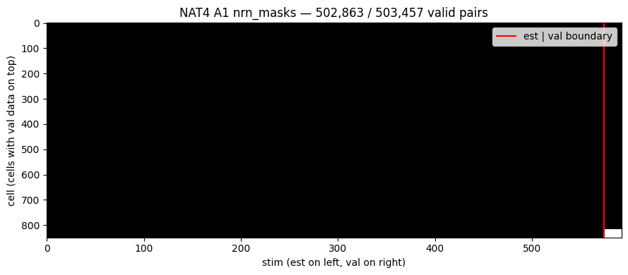
cells with ≥1 val response: 816 / 849
cells with NO val data:     33

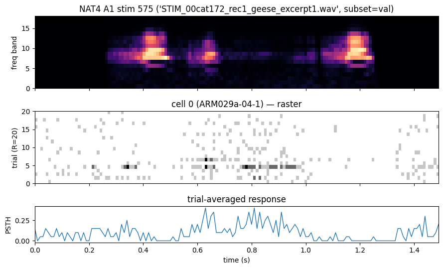
4. Stim metadata + one example stim/response

The estimation stims and validation stims share the same spectrogram-extraction pipeline; what differs is the trial count (typically 1 repeat for est vs ~10-20 for val). Below: a validation stim spectrogram and the response of one auditory cell.

# Find a val stim with a high-coverage auditory cell.
val_stim_indices = [s for s, m in enumerate(ds.stim_meta) if m['subset'] == 'val']
auditory_cell_indices = [i for i, n in enumerate(ds.nrn_meta) if n['auditory']]
for cell_idx in auditory_cell_indices:
    valid_val_stims = [s for s in val_stim_indices if not ds.responses[s][cell_idx].isnan().all()]
    if valid_val_stims:
        stim_idx = valid_val_stims[0]
        break

plot_stim_with_response(
    ds.stims[stim_idx], ds.responses[stim_idx][cell_idx], dt_ms=ds.dt,
    title=(f"NAT4 A1 stim {stim_idx} ('{ds.stim_meta[stim_idx]['name']}', "
           f"subset={ds.stim_meta[stim_idx]['subset']}) "
           f"→ cell {cell_idx} ({ds.nrn_meta[cell_idx]['cell_id']})"),
)
plt.show()

5. The bidirectional rule

select_stims_by_attr('subset', 'val') filters down to validation stims. Because we now restrict the stim set, neurons whose only valid responses lie outside the selection (i.e. the val-less cells visible in §3) are auto-hidden. This is the bidirectional rule from `data_paradigm.md <../docs/_source/md/data_paradigm.md>`__ §8: a stim selection implicitly induces a population selection.

After the selection:

• Stims drop from 593 to 18 (only validation stims remain).

• Cells drop from 849 to 816 (the 33 val-less cells are hidden).

ds.select_stims_by_attr('subset', 'val')

n_visible_cells = ds.nrn_masks.sum(dim=0).gt(0).sum().item() if ds.S_sel is None else len(ds._selected())
print(f"after select_stims_by_attr('subset', 'val'):")
print(f"  visible stims:  {len(ds.S_sel) if ds.S_sel is not None else len(ds.stims)}")
print(f"  visible cells:  {len(ds._selected())}")

# What __getitem__ returns now: only val-data cells, only val stims.
item = ds[0]
stim, responses_per_neuron, meta = item['stims'], item['responses'], item['stim_meta']
print(f"\nfirst returned item:")
print(f"  stim shape:  {tuple(stim.shape)}")
print(f"  N returned:  {len(responses_per_neuron)}")
print(f"  meta:        {meta}")

# undo selection so subsequent cells see the full dataset
ds.reset_stim_selection()
ds.reset_pop_selection()

after select_stims_by_attr('subset', 'val'):
  visible stims:  18
  visible cells:  816

first returned item:
  stim shape:  (1, 18, 150)
  N returned:  816
  meta:        {'name': 'STIM_00cat172_rec1_geese_excerpt1.wav', 'subset': 'val'}

6. Population filtering — select_pop_by_nrn_attr

The neuron-axis filters work on any key in nrn_meta. Two common cases: keeping only auditory cells, and slicing by animal / recording site.

ds.select_pop_by_nrn_attr('auditory', True)
print(f"after select_pop_by_nrn_attr('auditory', True): {len(ds._selected())} cells")
ds.reset_pop_selection()

ds.select_pop_by_nrn_attr('animal', 'ARM')
print(f"after select_pop_by_nrn_attr('animal', 'ARM'):  {len(ds._selected())} cells")
ds.reset_pop_selection()

after select_pop_by_nrn_attr('auditory', True): 777 cells
after select_pop_by_nrn_attr('animal', 'ARM'):  165 cells

7. The valid_mask from neural_collate

When the dataset feeds a DataLoader with neural_collate, the collator emits a fine-grained (B, N, R, T) bool mask alongside the NaN-padded responses tensor. Loss code uses this directly (see `metrics_paradigm.md <../docs/_source/md/metrics_paradigm.md>`__ §4) — no need to re-scan for NaN positions.

# small batched loader (val stims, restricted to auditory cells)
ds.select_stims_by_attr('subset', 'val')
ds.select_pop_by_nrn_attr('auditory', True)
loader = DataLoader(ds, batch_size=4, shuffle=False, collate_fn=neural_collate)
batch = next(iter(loader))
stims, responses, valid_mask, stim_metas = batch['stims'], batch['responses'], batch['valid_mask'], batch['stim_meta']
print(f"stims:      {tuple(stims.shape)}  (B, 1, F, T)")
print(f"responses:  {tuple(responses.shape)}  (B, N, R_max, T_max)")
print(f"valid_mask: {tuple(valid_mask.shape)}  bool")
print(f"NaN cells in responses: {responses.isnan().sum().item():,} / {responses.numel():,}")
print(f"valid_mask True count:  {valid_mask.sum().item():,}  (should equal numel - NaN count)")
ds.reset_stim_selection()
ds.reset_pop_selection()

stims:      (4, 1, 18, 150)  (B, 1, F, T)
responses:  (4, 744, 20, 150)  (B, N, R_max, T_max)
valid_mask: (4, 744, 20, 150)  bool
NaN cells in responses: 0 / 8,928,000
valid_mask True count:  8,928,000  (should equal numel - NaN count)

8. The PEG companion

NAT4 ships a second area, PEG (parabelt secondary auditory cortex). Same protocol, different population.

ds_peg = NAT4Dataset(area='PEG', download=True, subset='all')
print(f"PEG: {ds_peg.N_neurons} cells, {len(ds_peg.stims)} stims")
peg_auditory = sum(1 for n in ds_peg.nrn_meta if n['auditory'])
print(f"  auditory: {peg_auditory} / {ds_peg.N_neurons}")
peg_total = ds_peg.nrn_masks.sum().item()
peg_grid = ds_peg.nrn_masks.numel()
print(f"  coverage: {peg_total:,} / {peg_grid:,} valid pairs ({100*peg_total/peg_grid:.1f}%)")
print(f"  animals:  {dict(Counter(n['animal'] for n in ds_peg.nrn_meta))}")

/home/ulysse/miniconda3/envs/deepstrf_dev/lib/python3.11/site-packages/tqdm/auto.py:21: TqdmWarning: IProgress not found. Please update jupyter and ipywidgets. See https://ipywidgets.readthedocs.io/en/stable/user_install.html
  from .autonotebook import tqdm as notebook_tqdm
download PEG_NAT4_ozgf.fs100.ch18.tgz: 100%|██████████| 22.4M/22.4M [00:02<00:00, 10.4MB/s]
download PEG_pred_correlation.csv: 33.0kB [00:00, 959kB/s]
download PEG_single_sites.zip: 100%|██████████| 25.4M/25.4M [00:02<00:00, 12.6MB/s]
NAT4 PEG val sites: 100%|██████████| 12/12 [00:04<00:00,  2.98it/s]

PEG: 398 cells, 593 stims
  auditory: 339 / 398
  coverage: 236,014 / 236,014 valid pairs (100.0%)
  animals:  {'ARM': 398}

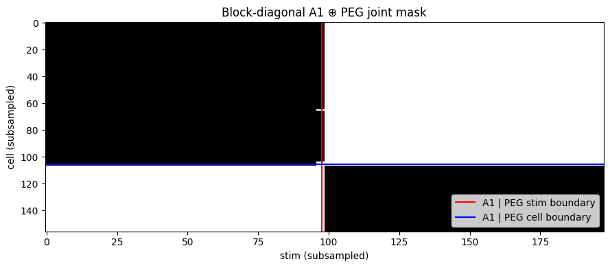
9. Cross-area concatenation

concat_neural_datasets([a1, peg]) builds a block-diagonal joint dataset along both stim and neuron axes — A1’s neurons see only A1’s stimuli (and vice versa) via NaN sentinels. A single population model over the union jointly fits both areas. See `dataset_concatenation.md <../docs/_source/md/dataset_concatenation.md>`__.

joint = concat_neural_datasets([ds, ds_peg])
print(f"joint dataset:")
print(f"  cells:  {joint.N_neurons}")
print(f"  stims:  {len(joint.stims)}")
joint_total = joint.nrn_masks.sum().item()
joint_grid = joint.nrn_masks.numel()
print(f"  coverage: {joint_total:,} / {joint_grid:,} valid pairs ({100*joint_total/joint_grid:.1f}%)")
print(f"  cross-area sanity: {ds.nrn_masks.sum().item() + ds_peg.nrn_masks.sum().item():,} == {joint_total:,}")

# verify the block-diagonal structure visually for a small subsample
fig, ax = plt.subplots(figsize=(9, 4))
sub = joint.nrn_masks[::6, ::8]    # every 6th stim, every 8th cell
ax.imshow(sub.numpy().T, aspect='auto', cmap='Greys', interpolation='nearest')
ax.axvline(len(ds.stims) // 6 - 0.5, color='red', lw=1.5, label='A1 | PEG stim boundary')
ax.axhline(ds.N_neurons // 8 - 0.5, color='blue', lw=1.5, label='A1 | PEG cell boundary')
ax.set_xlabel("stim (subsampled)")
ax.set_ylabel("cell (subsampled)")
ax.set_title("Block-diagonal A1 ⊕ PEG joint mask")
ax.legend(loc='lower right')
plt.tight_layout(); plt.show()

joint dataset:
  cells:  1247
  stims:  1186
  coverage: 738,877 / 1,478,942 valid pairs (50.0%)
  cross-area sanity: 738,877 == 738,877

What’s next

• End-to-end fit on NAT4 — the same Fitter/metrics stack from `fit_ns1_statenet.ipynb <fit_ns1_statenet.ipynb>`__ ports to NAT4 unchanged. The non-trivial bit is the est/val split: NAT4 already ships it, so use subset='est' for the train/val loaders and subset='val' for held-out evaluation.

• Cross-species pooling — replace the A1+PEG concat above with e.g. NS1+NAT4_A1 to fit ferret + ferret jointly, or with CRCNS_AA1 for cross-species.

• Stim selection tricks — the bidirectional rule (§5) makes per-stim-class evaluation a one-liner. Useful when reporting cc_norm on a particular stimulus class.