CRCNS AC1 — subthreshold Vm in rat auditory cortex (Wehr + Asari)

This notebook is a deep dive into the CRCNS AC1 dataset, which is special on two counts:

1. It is two published datasets in one container. The Wehr subset (Machens, Wehr & Zador 2004) and the Asari subset (Asari & Zador 2009) were recorded in the same lab and ship together in the CRCNS release. deepSTRF exposes both through a single CRCNSAC1Dataset, switchable with the experimenter= argument.

2. It is the only deepSTRF dataset with intracellular subthreshold membrane potential (Vm) for single units. Every other auditory dataset ships spike counts (non-negative). Here the default target is a signed, continuous voltage trace — action potentials were pharmacologically blocked in the Wehr recordings, so the subthreshold synaptic input is the whole signal.

We’ll show: the two subsets side by side, why subthreshold Vm needs different handling than spike counts, trial-to-trial variability, how the recording mode (whole-cell vs cell-attached) dictates whether the signal is subthreshold Vm or spikes, and the difference between Wehr fragments and Asari spliced sequences.

Setup — Google Colab

The cell below installs deepSTRF from source on Colab; on a local pip install -e . it’s a no-op.

Note on data. CRCNS AC1 is behind a free account. With download=True and $CRCNS_USERNAME / $CRCNS_PASSWORD set, the loader fetches the three archives (~1.6 GB) from the NERSC mirror and extracts them on first use. On a workstation with the data already unpacked, point CRCNS_AC1_DATA at the directory holding the zips / extracted folders.

import sys
if 'google.colab' in sys.modules:
    !pip install -q git+https://github.com/urancon/deepSTRF.git
    print('deepSTRF installed from GitHub.')
else:
    print('Local environment — assuming deepSTRF is already importable.')

Local environment — assuming deepSTRF is already importable.

Imports + paths

%matplotlib inline
import os
import warnings
from collections import Counter

import numpy as np
import matplotlib.pyplot as plt
import torch

from deepSTRF.datasets.audio import (
    CRCNSAC1Dataset, WEHR_VALID_NEURONS, WEHR_NEURONS_SPLIT_NATURAL,
)

# Where the CRCNS AC1 dump lives. None -> platformdirs cache (+ download=True).
DATA = os.environ.get('CRCNS_AC1_DATA', None)
DOWNLOAD = False  # flip to True on first run if the data isn't local

# A few repeats per cell get gated out as artifacts; that's expected, not a bug.
warnings.simplefilter('ignore')

1. The two subsets at a glance

experimenter= selects the subset; sites= selects A1 vs MGB (Wehr is all A1). We load the Wehr subset first — it’s small (25 cells, sf = 4 kHz) and loads in ~1 minute. The Asari subset comes later (it’s bigger and slower).

wehr = CRCNSAC1Dataset(path=DATA, download=DOWNLOAD,
                       experimenter='wehr', dt_ms=5.0)
print(f'WEHR : N={wehr.N_neurons}  S={len(wehr.stims)}  F={wehr.F}')
print(f'  spectrogram: {wehr.F} log-bands, {wehr.fmin:.0f}-{wehr.fmax:.0f} Hz, dt={wehr.dt} ms')
print(f'  signal_type: {wehr.signal_type!r}  (auto-derived from recording mode)')
print(f'  coverage (cells x stims that are real): '
      f'{wehr.nrn_masks.float().mean().item()*100:.0f}% dense')
print(f'  artifact-gated repeats: {wehr._rejection_counter}')

WEHR : N=25  S=51  F=53
  spectrogram: 53 log-bands, 100-45000 Hz, dt=5.0 ms
  signal_type: 'subthresh'  (auto-derived from recording mode)
  coverage (cells x stims that are real): 22% dense
  artifact-gated repeats: {'range': 1, 'step': 0, 'xcorr': 13, 'kept': 1249}

Each neuron is one whole-cell recording session; nrn_meta carries the provenance. Note the _wehr_cell_idx field — it indexes into the reproducibility constants used by Rançon et al. 2024/2025.

for m in wehr.nrn_meta[:3]:
    print({k: m[k] for k in ('experimenter','session','site','recording_type','_wehr_cell_idx')})
print('...')
print(f'\nWEHR_VALID_NEURONS  ({len(WEHR_VALID_NEURONS)} of 25 cells used in the papers):')
print(' ', WEHR_VALID_NEURONS)

{'experimenter': 'wehr', 'session': '20020508-mw-003', 'site': 'A1', 'recording_type': 'whole-cell', '_wehr_cell_idx': 0}
{'experimenter': 'wehr', 'session': '20020530-mw-001', 'site': 'A1', 'recording_type': 'whole-cell', '_wehr_cell_idx': 1}
{'experimenter': 'wehr', 'session': '20020602-mw-001', 'site': 'A1', 'recording_type': 'whole-cell', '_wehr_cell_idx': 2}
...

WEHR_VALID_NEURONS  (21 of 25 cells used in the papers):
  (0, 3, 5, 6, 7, 9, 10, 11, 12, 13, 14, 15, 16, 17, 18, 19, 20, 21, 22, 23, 24)

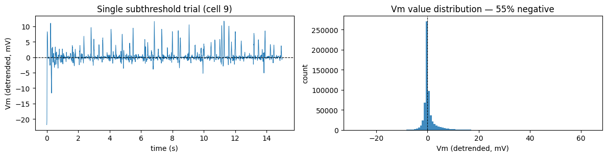
2. Subthreshold Vm is signed — unlike spike counts

Whole-cell recordings give the membrane potential after MedGauss drift removal (median + gaussian baseline subtracted). Because the baseline is removed, the trace oscillates around zero — roughly half the values are negative. Any loss / metric you apply must tolerate that: use MSE, not Poisson (which assumes non-negative rates).

For all the single-cell demos below we pick the (cell, stim) pair with the most repeated presentations — the clearest window onto trial-to-trial structure.

# Pick the (cell, stim) pair with the most repeats — the best trial-to-trial
# variability demo. Also note how many stims that cell heard overall.
best = max(
    ((wehr.responses[s][n].shape[0], n, s)
     for n in range(wehr.N_neurons) for s in range(len(wehr.stims))
     if wehr.nrn_masks[s, n]),
)
_, cell, demo_stim = best
stims_for_cell = [s for s in range(len(wehr.stims)) if wehr.nrn_masks[s, cell]]

resp = wehr.responses[demo_stim][cell].numpy()      # (R, T)
R, T = resp.shape
t_ax = np.arange(T) * wehr.dt / 1000.0
print(f'cell {cell}: {len(stims_for_cell)} stims; demo stim {demo_stim} '
      f"({wehr.stim_meta[demo_stim]['description']}) with R={R} trials")

# pool all this cell's Vm values to show the sign distribution
allvals = np.concatenate([wehr.responses[s][cell].numpy().ravel() for s in stims_for_cell])

fig, ax = plt.subplots(1, 2, figsize=(12, 3.2))
ax[0].plot(t_ax, resp[0], lw=0.7)
ax[0].axhline(0, color='k', lw=0.8, ls='--')
ax[0].set(title=f'Single subthreshold trial (cell {cell})',
          xlabel='time (s)', ylabel='Vm (detrended, mV)')
ax[1].hist(allvals, bins=120, alpha=0.85)
ax[1].axvline(0, color='k', lw=0.8, ls='--')
ax[1].set(title=f'Vm value distribution — {(allvals<0).mean()*100:.0f}% negative',
          xlabel='Vm (detrended, mV)', ylabel='count')
fig.tight_layout(); plt.show()

cell 9: 10 stims; demo stim 5 (knudsens frog) with R=25 trials

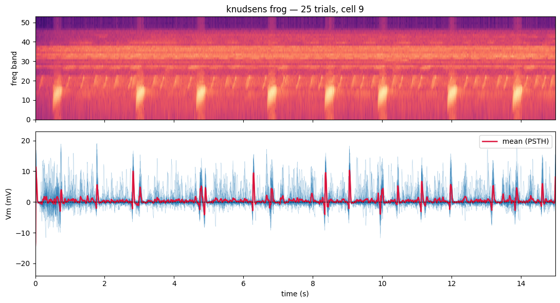
3. Trial-to-trial variability

Whole-cell Vm is remarkably reliable across repeats — the stimulus-locked deflections line up trial after trial, while a smaller fraction of the variance is trial-specific. Overlaying all R trials (thin) against their mean / PSTH (thick) gives a quick visual read on the SNR of a cell. This is exactly what the Sahani-Linden SNR (compute_neuron_quality()) quantifies.

spec = wehr.stims[demo_stim][0].numpy()       # (F, T)
mean_trace = resp.mean(0)

fig, ax = plt.subplots(2, 1, figsize=(11, 6), sharex=True,
                       gridspec_kw={'height_ratios': [1, 1.4]})
ax[0].imshow(spec, aspect='auto', origin='lower', cmap='magma',
             extent=[0, t_ax[-1], 0, wehr.F])
ax[0].set(ylabel='freq band',
          title=f"{wehr.stim_meta[demo_stim]['description']} — {R} trials, cell {cell}")
for r in range(R):
    ax[1].plot(t_ax, resp[r], lw=0.4, color='C0', alpha=0.35)
ax[1].plot(t_ax, mean_trace, lw=1.8, color='crimson', label='mean (PSTH)')
ax[1].axhline(0, color='k', lw=0.6, ls='--')
ax[1].set(xlabel='time (s)', ylabel='Vm (mV)')
ax[1].legend(loc='upper right')
fig.tight_layout(); plt.show()

4. The recording mode determines the signal (subthreshold vs spikes)

deepSTRF does not let you pick the signal type by hand — it’s dictated by how each cell was recorded, because the recording mode decides what signal physically exists:

recording mode	subset	signal (nrn_meta['signal_type'])	sign	pair with
whole-cell	Wehr, Asari A1	'subthresh' — MedGauss-detrended Vm	signed	mse_loss
cell-attached	Asari MGB	'spikes' — Hann-smoothed spike-rate	≥ 0	poisson_loss

Cell-attached recordings (MGB) have no intracellular Vm at all — the trace is dominated by extracellular action potentials. Whole-cell recordings (Wehr, Asari A1) carry subthreshold Vm and no spikes (blocked in Wehr, not analysed in Asari A1). So the right target is fixed by the data, and the loader sets it automatically.

To see real spikes we load the Asari MGB cohort (cell-attached). This is a few-minute load.

mgb = CRCNSAC1Dataset(path=DATA, download=DOWNLOAD,
                      experimenter='asari', sites='MGB', dt_ms=5.0)
print(f'ASARI MGB : N={mgb.N_neurons}  signal_type={mgb.signal_type!r}  '
      f"rec={set(m['recording_type'] for m in mgb.nrn_meta)}")

# A spike-rate PSTH from one MGB cell, next to the Wehr subthreshold Vm.
m_cell = int(mgb.nrn_masks.sum(0).argmax())
m_stims = [s for s in range(len(mgb.stims)) if mgb.nrn_masks[s, m_cell]]
m_stim = max(m_stims, key=lambda s: mgb.responses[s][m_cell].shape[0])
m_resp = mgb.responses[m_stim][m_cell].numpy()
m_psth = m_resp.mean(0)
m_t = np.arange(m_psth.size) * mgb.dt / 1000.0
# mean evoked rate sanity check (Asari 2009 report ~11 Hz evoked in MGB)
mean_rate_hz = m_psth.mean() / (mgb.dt / 1000.0)
print(f'  MGB cell {m_cell}: R={m_resp.shape[0]} trials, mean rate ~{mean_rate_hz:.0f} a.u./s')

fig, ax = plt.subplots(2, 1, figsize=(11, 5), sharex=False)
ax[0].plot(t_ax[:len(mean_trace)], mean_trace, color='C0')
ax[0].axhline(0, color='k', lw=0.6, ls='--')
ax[0].set(ylabel='Vm (mV)', xlabel='time (s)',
          title="whole-cell (Wehr A1) -> 'subthresh': signed membrane potential")
ax[1].plot(m_t, m_psth, color='C3')
ax[1].set(ylabel='rate (a.u.)', xlabel='time (s)',
          title="cell-attached (Asari MGB) -> 'spikes': Hann-smoothed rate (>= 0)")
fig.tight_layout(); plt.show()
print(f'subthresh min = {mean_trace.min():+.2f} mV   |   MGB spikes min = {m_psth.min():.2f} (a.u.)')

ASARI MGB : N=14  signal_type='spikes'  rec={'cell-attached'}
  MGB cell 1: R=23 trials, mean rate ~85 a.u./s

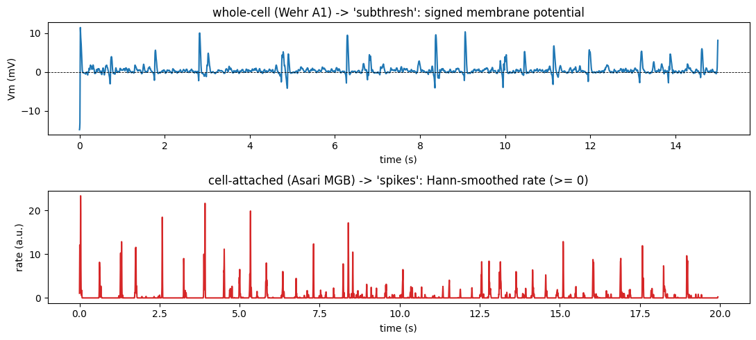
subthresh min = -14.78 mV   |   MGB spikes min = 0.00 (a.u.)

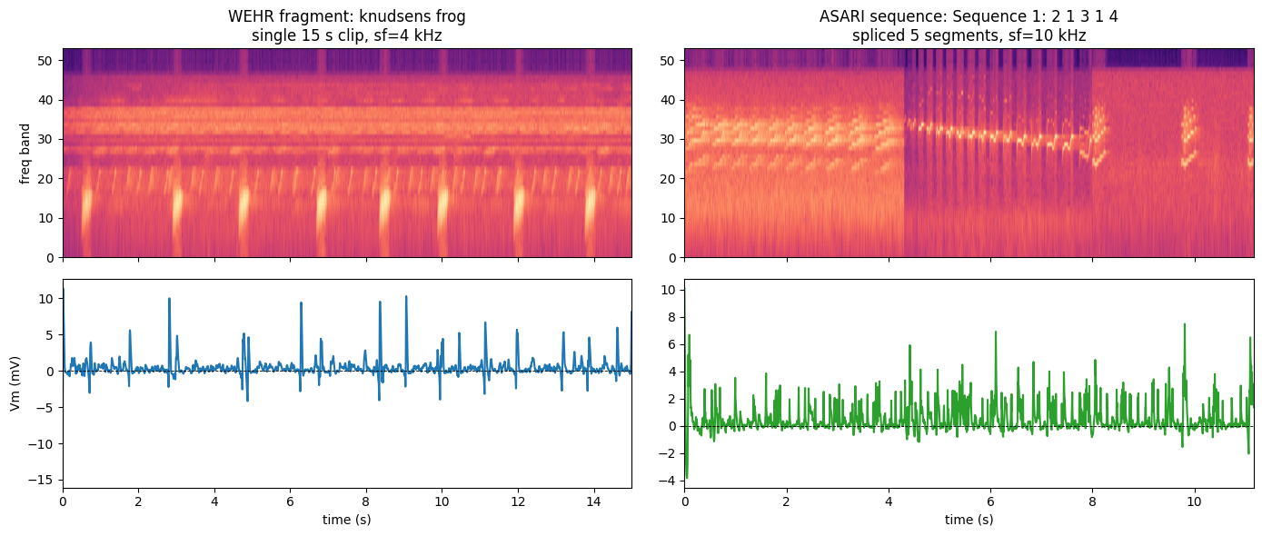
5. Wehr fragments vs Asari spliced sequences

The two subsets differ in their stimulus design, which the loader surfaces in stim_meta:

• Wehr plays single 15 s natural-sound fragments (humpback whale, jaguar mating call, …) at sf = 4 kHz.

• Asari plays sequences that splice 5 short segments together (e.g. 'Sequence 1: 2 1 3 1 4') at sf = 10 kHz, to probe long-range context dependence. The loader resolves each sequence to the exact segment files and records them in stim_meta['segment_files'].

Here we load the Asari A1 cohort so both panels show subthreshold Vm — isolating the stimulus difference from the signal-type difference of §4. Like the MGB load, this takes a few minutes (39 whole-cell recordings at 10 kHz).

asari = CRCNSAC1Dataset(path=DATA, download=DOWNLOAD,
                        experimenter='asari', sites='A1', dt_ms=5.0)
print(f'ASARI A1 : N={asari.N_neurons}  S={len(asari.stims)}  F={asari.F}')
print(f'  artifact-gated repeats: {asari._rejection_counter}')

a_cell = int(asari.nrn_masks.sum(0).argmax())
a_stims = [s for s in range(len(asari.stims)) if asari.nrn_masks[s, a_cell]]
a_stim = max(a_stims, key=lambda s: asari.responses[s][a_cell].shape[0])
sm = asari.stim_meta[a_stim]
print(f"  demo sequence: {sm['sequence']}")
print(f"  spliced from: {sm['segment_files']}")

ASARI A1 : N=39  S=67  F=53
  artifact-gated repeats: {'range': 0, 'step': 0, 'xcorr': 18, 'kept': 1859}
  demo sequence: Sequence 1: 2 1 3 1 4
  spliced from: ('class4/6.mat', 'class4/5.mat', 'class4/7.mat', 'class4/5.mat', 'class4/8.mat')

a_spec = asari.stims[a_stim][0].numpy()
a_resp = asari.responses[a_stim][a_cell].numpy().mean(0)
a_t = np.arange(a_spec.shape[1]) * asari.dt / 1000.0

fig, ax = plt.subplots(2, 2, figsize=(14, 6), sharex='col')
ax[0,0].imshow(spec, aspect='auto', origin='lower', cmap='magma',
               extent=[0, t_ax[-1], 0, wehr.F])
ax[0,0].set(ylabel='freq band',
            title=f"WEHR fragment: {wehr.stim_meta[demo_stim]['description']}\n"
                  f'single 15 s clip, sf=4 kHz')
ax[1,0].plot(t_ax, mean_trace, color='C0'); ax[1,0].axhline(0, color='k', lw=0.6, ls='--')
ax[1,0].set(xlabel='time (s)', ylabel='Vm (mV)')
ax[0,1].imshow(a_spec, aspect='auto', origin='lower', cmap='magma',
               extent=[0, a_t[-1], 0, asari.F])
ax[0,1].set(title=f"ASARI sequence: {sm['sequence']}\n"
                  f"spliced {len(sm['segments'])} segments, sf=10 kHz")
ax[1,1].plot(a_t, a_resp, color='C2'); ax[1,1].axhline(0, color='k', lw=0.6, ls='--')
ax[1,1].set(xlabel='time (s)')
fig.tight_layout(); plt.show()

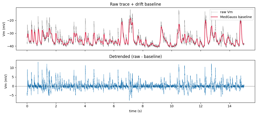
6. Under the hood — MedGauss detrend + artifact gating

Intracellular recordings drift (slow baseline wander) and occasionally jump (electrode movement, dropouts). The loader handles both before you ever see the data:

1. MedGauss detrend — subtract a median-then-gaussian low-pass baseline (100 ms median, 10 ms σ), removing drift while preserving fast Vm dynamics.

2. Per-repeat gating (RepeatGating) — drop trials that clip the amplifier range, sit on a sustained baseline step (movement / dropout the baseline can’t track), or disagree with their peers (low cross-trial correlation).

The raw traces aren’t on the public dataset (only the cleaned responses are), but we can call the native ingest helpers to visualise one raw trial, its baseline, and the detrended result.

from deepSTRF.datasets.audio._crcns_ac1_native import (
    ensure_extracted, iterate_wehr_cells, medgauss_detrend,
)

wehr_dir, _, _ = ensure_extracted(wehr.path)
raw_cell = next(iterate_wehr_cells(wehr_dir))   # first session
raw_stim = raw_cell.stims[0]
raw = raw_stim.raw_repeats[0]                    # one raw Vm trial (mV, sf=4kHz)
sf = raw_stim.sf_resp
detr = medgauss_detrend(raw, sf)
baseline = raw - detr
tt = np.arange(raw.size) / sf

fig, ax = plt.subplots(2, 1, figsize=(11, 5), sharex=True)
ax[0].plot(tt, raw, lw=0.5, color='gray', label='raw Vm')
ax[0].plot(tt, baseline, lw=1.5, color='crimson', label='MedGauss baseline')
ax[0].legend(loc='upper right'); ax[0].set(ylabel='Vm (mV)', title='Raw trace + drift baseline')
ax[1].plot(tt, detr, lw=0.5, color='C0'); ax[1].axhline(0, color='k', lw=0.6, ls='--')
ax[1].set(xlabel='time (s)', ylabel='Vm (mV)', title='Detrended (raw - baseline)')
fig.tight_layout(); plt.show()

print('Repeats kept vs rejected, by reason:')
print('  WEHR    :', wehr._rejection_counter)
print('  ASARI A1:', asari._rejection_counter)

Repeats kept vs rejected, by reason:
  WEHR    : {'range': 1, 'step': 0, 'xcorr': 13, 'kept': 1249}
  ASARI A1: {'range': 0, 'step': 0, 'xcorr': 18, 'kept': 1859}

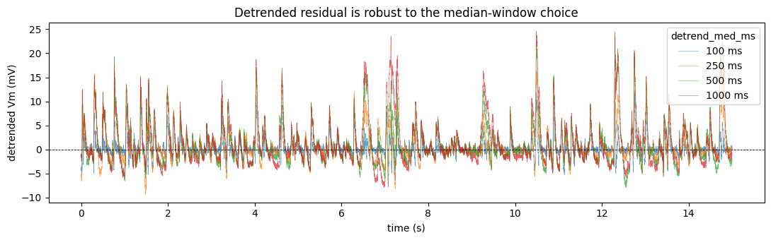
The median window (detrend_med_ms, default 100 ms) is a constructor argument. It barely matters here: because the response is dominated by fast PSP transients (much shorter than 100 ms), the detrended residual is almost identical from 100 ms up to 1 s. Longer windows preserve marginally more slow Vm dynamics; shorter windows detrend more aggressively.

fig, ax = plt.subplots(figsize=(11, 3.5))
for med in (100, 250, 500, 1000):
    ax.plot(tt, medgauss_detrend(raw, sf, med_ms=med), lw=0.4, alpha=0.7, label=f'{med} ms')
ax.axhline(0, color='k', lw=0.6, ls='--')
ax.set(xlabel='time (s)', ylabel='detrended Vm (mV)',
       title='Detrended residual is robust to the median-window choice')
ax.legend(title='detrend_med_ms'); fig.tight_layout(); plt.show()

7. Filtering + reproducibility constants

The standard deepSTRF filter API works on both subsets. Because they share a class, you can also load both at once and split by experimenter / site. For the Rançon et al. STRF baseline, reduce to the published cell list and per-neuron split with the two exported constants.

# Load BOTH subsets in one object, then split by experimenter.
# (Asari MGB is included here; this is the full-dataset load.)
# both = CRCNSAC1Dataset(path=DATA, download=DOWNLOAD, dt_ms=5.0)  # ~12 min
# print('combined N =', both.N_neurons)

# Reproducibility: keep only the 21 published Wehr cells.
keep = wehr.select_pop_by_nrn_predicate(
    lambda n: n['_wehr_cell_idx'] in WEHR_VALID_NEURONS
)
print(f'kept {len(keep)} of {wehr.N_neurons} Wehr cells (the published cohort)')

# Their (train, val, test) stim-count splits used in the papers:
for n in keep[:5]:
    idx = wehr.nrn_meta[n]['_wehr_cell_idx']
    print(f"  cell_idx {idx:2d}: split (train,val,test) = {WEHR_NEURONS_SPLIT_NATURAL[idx]}")

kept 21 of 25 Wehr cells (the published cohort)
  cell_idx  0: split (train,val,test) = (7, 2, 2)
  cell_idx  3: split (train,val,test) = (7, 1, 1)
  cell_idx  5: split (train,val,test) = (6, 1, 1)
  cell_idx  6: split (train,val,test) = (3, 1, 1)
  cell_idx  7: split (train,val,test) = (1, 1, 1)

What’s next

• STRF / LN baselines. The Fitter (see docs/_source/md/fitter.md) ports unchanged. For the whole-cell subthreshold cohorts pair it with mse_loss; for the cell-attached MGB spikes (sites='MGB') pair with poisson_loss. Don’t mix the two cohorts under one model — they’re in different units (the loader warns you if you load both).

• Per-cell quality. Call ds.compute_neuron_quality() to write Sahani-Linden snr + Hsu/Spearman-Brown ccmax into nrn_meta, then filter on them (select_pop_by_nrn_predicate(lambda n: n['snr'] > 0.5)).

• Wehr-2024 spectrogram layout. Pass fmax=25600.0 to recover the 49-band setting (vs the 53-band Asari-2025 default used here).

• Tune the detrend. detrend_med_ms (default 100 ms) sets the MedGauss median window; raise it to preserve more slow Vm dynamics, lower it to detrend more aggressively. The choice is robust — residuals barely change between 100 and 1000 ms because fast PSP transients dominate the response.

• Reproduce the paper numbers. On the published Wehr cohort, a StateNet-GRU reaches cc_norm ≈ 0.31 and a Linear STRF ≈ 0.21 (population means, Rançon et al. 2025 Table 1). For the Linear model use temporal_window_size ≈ 20–40 at dt_ms=5.0 (a 100–200 ms window) — a stateless STRF needs the long window to reach that score; the GRU gets its temporal context from recurrence (T=1 input).