STRF parameterizations — same data, same model, different inductive bias

This notebook fits a Linear STRF model on NS1 with three different kernel parameterizations of the spectro-temporal receptive field, all else equal:

1. Vanilla ``nn.Conv2d`` — the textbook unconstrained STRF. Every (F, T) cell of the kernel is a free parameter.

2. ``SeparableSTRF`` — frequency-time separable, rank-1. The kernel factorises as w_F(f) · w_T(t), drastically reducing the parameter count.

3. ``ParametricSTRF`` — sum of K learnable 2D Gaussians (DCLS-style; see DCLS asymmetric-kernel bug note for why deepSTRF reimplements rather than wraps the upstream library).

Same NS1 split (14 train / 3 val / 3 test), same Fitter settings, same seed. The questions:

• How does mean test cc_norm compare?

• For a cell that fits well across all three, what do the learned STRFs look like? Where do the inductive biases pull the kernel?

Note on runtime: three end-to-end fits at 100 epochs each on a consumer GPU. Around 25 min total.

Setup — Google Colab

If you’re running on Google Colab, the cell below installs deepSTRF from source. On a local install (pip install -e .) it’s a no-op.

import sys
if 'google.colab' in sys.modules:
    !pip install -q git+https://github.com/urancon/deepSTRF.git
    print("deepSTRF installed from GitHub.")
else:
    print("Local environment — assuming deepSTRF is already importable.")

Imports

%matplotlib inline
from collections import OrderedDict
import time
import matplotlib.pyplot as plt
import numpy as np
import torch
import torch.nn as nn
from torch.utils.data import DataLoader, Subset

from deepSTRF.datasets.audio.ns1 import NS1Dataset
from deepSTRF.models.audio import Linear
from deepSTRF.models.layers import ParametricSTRF, SeparableSTRF
from deepSTRF.training import Fitter, set_random_seed
from deepSTRF.utils import neural_collate, plot_strf_grid

device = "cuda" if torch.cuda.is_available() else "cpu"
print(f"Using device: {device}")

1. Load NS1 and set up the same train / val / test split

ds = NS1Dataset(dt_ms=5.0, smooth=True, download=True)
F = 34          # spectrogram frequency bands
T_strf = 15     # STRF temporal extent (frames at dt=5 ms → 75 ms history)
N = ds.N_neurons

train_loader = DataLoader(Subset(ds, list(range(14))),    batch_size=1, shuffle=True,  collate_fn=neural_collate)
val_loader   = DataLoader(Subset(ds, list(range(14, 17))), batch_size=1, shuffle=False, collate_fn=neural_collate)
test_loader  = DataLoader(Subset(ds, list(range(17, 20))), batch_size=1, shuffle=False, collate_fn=neural_collate)

print(f"NS1: N={N} cells | F={F} bands | dt=5 ms | T_strf={T_strf} frames")

NS1: N=119 cells | F=34 bands | dt=5 ms | T_strf=15 frames

2. A small fit-and-extract helper

One function that:

• Builds a Linear(F, T_strf, N, kernel=...) model with the chosen STRF parameterization.

• Trains for 50 epochs with the canonical Fitter defaults.

• Returns the training history, test metrics, and the learned STRF weights for every cell ((N, F, T) tensor — see model_paradigm.md §9).

def fit_with_kernel(name, build_kernel_fn, max_epochs=100, seed=0):
    set_random_seed(seed)
    kernel = build_kernel_fn()
    model = Linear(n_frequency_bands=F, temporal_window_size=T_strf,
                   out_neurons=N, kernel=kernel)
    n_params = model.count_trainable_params()
    print(f"  {name:20s} | params/neuron: {n_params // N:>5,d} (total {n_params:,})", flush=True)
    optimizer = torch.optim.AdamW(model.parameters(), lr=1e-3, weight_decay=0.0)
    fitter = Fitter(model, train_loader, val_loader,
                    optimizer=optimizer, device=device,
                    max_epochs=max_epochs, patience=max_epochs,   # disable early stop for fair compare
                    monitor="val_cc_norm", mode="max",
                    log_fn=lambda d: None)
    t0 = time.time()
    history = fitter.fit()
    elapsed = time.time() - t0
    test_metrics = fitter.evaluate(test_loader)
    strfs = model.STRF_weight().cpu()                      # (N, F, T)
    return {
        "name": name,
        "history": history,
        "test_cc": test_metrics["cc"].cpu(),
        "test_cc_norm": test_metrics["cc_norm"].cpu(),
        "strfs": strfs,
        "n_params": n_params,
        "elapsed": elapsed,
    }

3. Three fits

Same NS1 split, same Fitter settings, three different kernels.

results = OrderedDict()
print("Fitting Linear with three STRF parameterizations on NS1 ...")
results["vanilla"]    = fit_with_kernel("vanilla Conv2d", lambda: None)
results["separable"]  = fit_with_kernel("SeparableSTRF",  lambda: SeparableSTRF(F, T_strf, C_in=1, C_out=N))
results["parametric"] = fit_with_kernel("ParametricSTRF (8G)", lambda: ParametricSTRF(F, T_strf, C_in=1, C_out=N, num_gaussians=8))

Fitting Linear with three STRF parameterizations on NS1 ...
  vanilla Conv2d       | params/neuron:   511 (total 60,877)
  SeparableSTRF        | params/neuron:    50 (total 6,018)
  ParametricSTRF (8G)  | params/neuron:    41 (total 4,947)

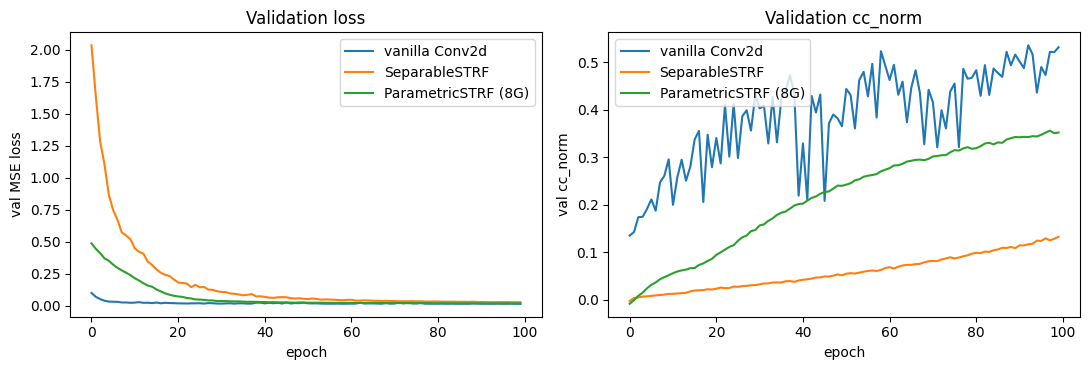
4. Side-by-side training curves

fig, axs = plt.subplots(1, 2, figsize=(11, 3.8))
for key, r in results.items():
    epochs = [h["epoch"] for h in r["history"]]
    val_loss = [h["val_loss"] for h in r["history"]]
    val_ccn  = [torch.nanmean(h["val_cc_norm"]).item() for h in r["history"]]
    axs[0].plot(epochs, val_loss, label=r["name"], lw=1.5)
    axs[1].plot(epochs, val_ccn,  label=r["name"], lw=1.5)
axs[0].set_xlabel("epoch"); axs[0].set_ylabel("val MSE loss"); axs[0].legend(); axs[0].set_title("Validation loss")
axs[1].set_xlabel("epoch"); axs[1].set_ylabel("val cc_norm");   axs[1].legend(); axs[1].set_title("Validation cc_norm")
plt.tight_layout(); plt.show()

5. Test-set metrics + parameter-count summary

print(f"{'parameterization':<22s} {'params/neuron':>14s}  {'total':>9s}  {'fit (s)':>8s}  {'test cc (mean)':>16s}  {'test cc_norm (mean)':>22s}")
print("-" * 95)
for r in results.values():
    print(f"{r['name']:<22s} {r['n_params'] // N:>14,d}  {r['n_params']:>9,}  {r['elapsed']:>8.1f}  "
          f"{torch.nanmean(r['test_cc']):>+16.3f}  {torch.nanmean(r['test_cc_norm']):>+22.3f}")

parameterization        params/neuron      total   fit (s)    test cc (mean)     test cc_norm (mean)
-----------------------------------------------------------------------------------------------
vanilla Conv2d                    511     60,877     484.7            +0.523                  +0.609
SeparableSTRF                      50      6,018     522.7            +0.159                  +0.184
ParametricSTRF (8G)                41      4,947     517.8            +0.383                  +0.445

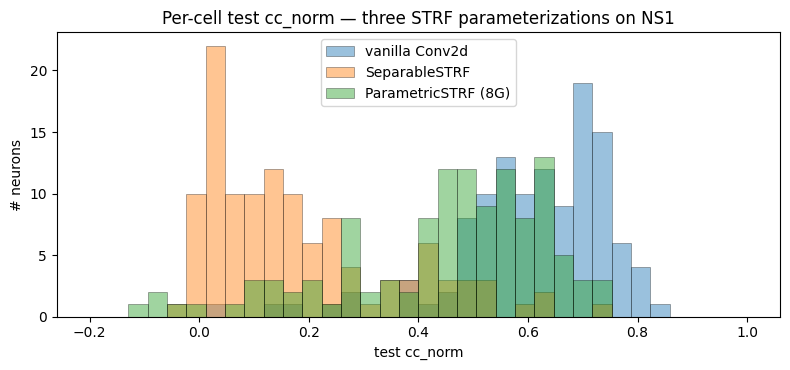
6. Per-cell test cc_norm distributions

fig, ax = plt.subplots(figsize=(8, 3.8))
bins = np.linspace(-0.2, 1.0, 35)
for key, r in results.items():
    ax.hist(r["test_cc_norm"].numpy(), bins=bins, alpha=0.45, label=r["name"], edgecolor="black", linewidth=0.5)
ax.set_xlabel("test cc_norm")
ax.set_ylabel("# neurons")
ax.set_title("Per-cell test cc_norm — three STRF parameterizations on NS1")
ax.legend()
plt.tight_layout(); plt.show()

7. Pick a well-fit cell, compare STRFs side by side

We pick the neuron whose mean test cc_norm across the three parameterizations is highest — i.e. a cell that all three models can fit reasonably. The three STRFs for that cell are plotted on the same colour scale.

ccn_stack = torch.stack([r["test_cc_norm"] for r in results.values()])    # (3, N)
mean_per_cell = torch.nanmean(ccn_stack, dim=0)
best_cell = int(torch.argmax(mean_per_cell).item())
print(f"Best-fit cell across the three parameterizations: idx={best_cell}")
for r in results.values():
    print(f"  {r['name']:<22s} test cc_norm = {r['test_cc_norm'][best_cell]:+.3f}")

Best-fit cell across the three parameterizations: idx=49
  vanilla Conv2d         test cc_norm = +0.807
  SeparableSTRF          test cc_norm = +0.647
  ParametricSTRF (8G)    test cc_norm = +0.697

strfs_for_best = [r["strfs"][best_cell].numpy() for r in results.values()]   # 3 × (F, T)
titles = [f"{r['name']}\ncc_norm = {r['test_cc_norm'][best_cell]:+.3f}"
          for r in results.values()]

plot_strf_grid(
    strfs_for_best, titles=titles, dt_ms=5, ncols=3, shared_clim=True,
    suptitle=f"Cell idx={best_cell}: same neuron, same data, three inductive biases",
    figsize=(11, 3.5),
)
plt.show()

Reading the result

These vanilla-Linear numbers are in the literature range for NS1 (Rancon et al. 2025, Comms. Biol. report >0.5 mean cc_norm on the NS1 Linear baseline). Compared to the StateNet GRU fit on the same split (`fit_ns1_statenet.ipynb <fit_ns1_statenet.ipynb>`__, cc_norm ≈ 0.77), Linear leaves headroom on the table — that’s exactly the gap a recurrent / feed-forward nonlinearity can recover.

The interesting comparison is the inductive-bias trade-off:

• Vanilla Conv2d (511 params/neuron) wins on absolute cc_norm — the unconstrained (F, T) kernel can carve out arbitrary spectro-temporal patterns.

• ParametricSTRF (41 params/neuron, 8 Gaussians) trails modestly with ~12× fewer parameters per neuron. The Gaussian-mixture parameterization is a strong prior for STRFs that look like spectrally-localised excitation/inhibition pairs — common in auditory cortex.

• SeparableSTRF (50 params/neuron, rank-1) collapses well below the other two. The rank-1 constraint w_F(f) · w_T(t) forces the kernel to be a single frequency profile multiplied by a single temporal profile — too restrictive for cells whose spectro-temporal response evolves through time (e.g. excitatory band early followed by inhibition at a different band).

What’s next

• AdapTrans prefilter — a learnable cochlear-adaptation front-end that often improves mean cc_norm on auditory data; pairs with any of the three STRF parameterizations above.

• Gradmaps — an architecture-agnostic alternative to closed-form STRF extraction, computed via gradient-of-output-vs-input. Useful for models without a pluggable kernel (DNet, ConvNet2D, StateNet, …).