Encoding zebra finch auditory pallium responses to unoccluded song

End-to-end demo of ``Le2025Dataset`` (Le, Bjoring & Meliza 2025, Nat Commun; DOI, figshare) → StateNet GRU → cc / cc_norm benchmark.

The Le 2025 dataset contains responses of single units in the zebra finch auditory pallium to 8 conspecific song motifs in up to 7 variants per critical interval — the variants are how the paper probes the auditory restoration illusion. For this baseline encoding fit, we use only the unoccluded ``C`` (Continuous) variant of each motif: 8 stims × 10 reps of clean natural song. That is the natural control for a stimulus-to-PSTH encoding model — directly comparable to AA1 / NS1 / NAT4 benchmarks.

Pipeline:

1. Load the nat8b sub-experiment (cohort 3, 445 units, full variant set).

2. Restrict to the 8 unoccluded C stims with ds.select_variant('C').

3. Split 6 / 1 / 1 motifs train / val / test.

4. Fit a StateNet GRU population model (one model jointly fits all 445 cells).

5. Report Pearson cc and noise-corrected cc_norm on the held-out motif.

6. (Bonus) Use the fitted model to predict responses to the occluded variants — a first qualitative look at whether the encoding model sees “restoration” in its outputs.

Setup — Google Colab

If you’re on Colab, the cell below installs deepSTRF + the gammatone extra (needed to compute the paper’s spectrograms). On a local install (pip install -e ".[le]") it’s a no-op.

The ~3 GB Le 2025 figshare archive is auto-downloaded on first use (download=True in the constructor — pulled from figshare, unpacked into the platformdirs cache; override via $DEEPSTRF_DATA_DIR).

import sys
if 'google.colab' in sys.modules:
    !pip install -q 'git+https://github.com/urancon/deepSTRF.git#egg=deepSTRF[le]'
    print('deepSTRF[le] installed from GitHub.')
else:
    print('Local environment — assuming deepSTRF + gammatone are importable.')

Local environment — assuming deepSTRF + gammatone are importable.

Imports

%matplotlib inline
import matplotlib.pyplot as plt
import numpy as np
import torch
from torch.utils.data import DataLoader, Subset

from deepSTRF.datasets.audio import Le2025Dataset
from deepSTRF.models.audio import StateNet
from deepSTRF.training import Fitter, set_random_seed
from deepSTRF.utils.data import neural_collate

device = 'cuda' if torch.cuda.is_available() else 'cpu'
print(f'Using device: {device}')
set_random_seed(0)

Using device: cuda

1. Load Le 2025 — nat8b sub-experiment

Le2025Dataset computes the paper-faithful gammatone spectrogram (50 log-spaced bands, 1–8 kHz, 2.5 ms window, 1 ms hop, log(P+1) compression — Methods p. 10). We use dt_ms=5 here for speed; pass dt_ms=1 for an exact paper-matched binning.

ds = Le2025Dataset(
    download=True,
    experiment='nat8b',   # cohort 3, natural-syntax motifs, full variant set
    dt_ms=5.0,            # paper uses 1 ms; 5 ms keeps the demo brisk
    smooth=True,
)
print(f'Total stims:    {len(ds.stim_meta)}    (8 motifs × 12 variants)')
print(f'Total neurons:  {ds.N_neurons}')
print(f'Bands × hop:    {ds.F} × {ds.dt} ms')
print(f'Variants on disk: {sorted({m["variant"] for m in ds.stim_meta})}')
print(f'Motifs on disk:   {sorted({m["motif"] for m in ds.stim_meta})}')

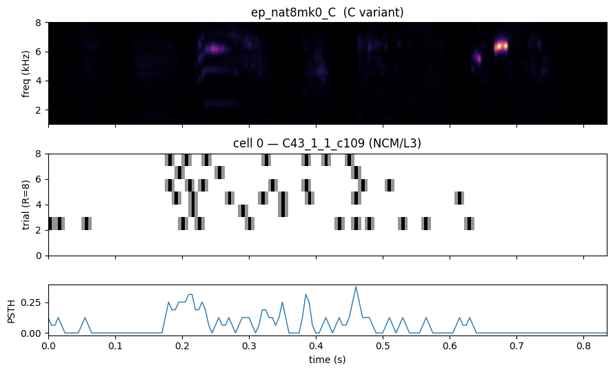
2. Quick look — one motif, one cell

The gammatone spectrogram below is the unmodified motif (C variant); the raster underneath is one cell’s repeats and the trial-averaged PSTH.

stim_idx = next(i for i, m in enumerate(ds.stim_meta)
                if m['motif'] == 'nat8mk0' and m['variant'] == 'C')
cell_idx = 0

spec = ds.stims[stim_idx][0].numpy()
resp = ds.responses[stim_idx][cell_idx].numpy()
psth = resp.mean(axis=0)
t = np.arange(spec.shape[1]) * ds.dt * 1e-3

fig, axs = plt.subplots(3, 1, figsize=(9, 5.5), sharex=True,
                        gridspec_kw={'height_ratios': [2, 2, 1]})
axs[0].imshow(spec, aspect='auto', origin='lower', cmap='magma',
              extent=[t[0], t[-1], ds.fmin/1000, ds.fmax/1000])
axs[0].set_ylabel('freq (kHz)')
axs[0].set_title(f"{ds.stim_meta[stim_idx]['name']}  ({ds.stim_meta[stim_idx]['variant']} variant)")

axs[1].imshow(resp, aspect='auto', cmap='Greys',
              extent=[t[0], t[-1], 0, resp.shape[0]])
axs[1].set_ylabel(f'trial (R={resp.shape[0]})')
axs[1].set_title(f'cell {cell_idx} — {ds.nrn_meta[cell_idx]["cell_id"]} ({ds.nrn_meta[cell_idx]["area"]})')

axs[2].plot(t, psth, lw=1.0)
axs[2].set_ylabel('PSTH')
axs[2].set_xlabel('time (s)')
plt.tight_layout()
plt.show()

3. Restrict to unoccluded motifs and split by motif

select_variant('C') keeps the 8 unmodified motifs and (via the bidirectional rule on nrn_masks) drops any neurons that lacked C-variant data. We then split motif-wise: 6 train / 1 val / 1 test.

Why split by motif rather than by trial? Trials of the same motif are near-identical noise realizations of the same stimulus; splitting trials leaks the stim distribution into val/test. Motif-wise split gives a true held-out generalization test.

ds.select_variant('C')
print(f'After select_variant("C"):  len(ds)={len(ds)}  N selected={len(ds._selected())}')

# 8 motifs in canonical order; reproducibility via fixed seed.
motif_order = [m['motif'] for m in ds.stim_meta if m['variant'] == 'C']
C_stim_indices = [i for i, m in enumerate(ds.stim_meta) if m['variant'] == 'C']
print('C-variant motifs:', motif_order)

train_iter = list(range(6))     # the first 6 motifs
val_iter   = [6]                # 7th motif
test_iter  = [7]                # 8th motif

train_loader = DataLoader(Subset(ds, train_iter), batch_size=1, shuffle=True,  collate_fn=neural_collate)
val_loader   = DataLoader(Subset(ds, val_iter),   batch_size=1, shuffle=False, collate_fn=neural_collate)
test_loader  = DataLoader(Subset(ds, test_iter),  batch_size=1, shuffle=False, collate_fn=neural_collate)
print(f'train: {len(train_loader.dataset)} motifs, val: {len(val_loader.dataset)}, test: {len(test_loader.dataset)}')

After select_variant("C"):  len(ds)=8  N selected=445
C-variant motifs: ['nat8mk0', 'nat8mk1', 'nat8mk2', 'nat8mk3', 'nat8mk4', 'nat8mk5', 'nat8mk6', 'nat8mk7']
train: 6 motifs, val: 1, test: 1

4. Standardize the spectrograms

Per-band mean/std computed on train + val and applied to all stims (prevents test-stats leakage; see standardize_stims docstring).

ds.standardize_stims(stim_indices=[C_stim_indices[i] for i in train_iter + val_iter])
print('post-norm stim[0] min/mean/max:',
      ds.stims[C_stim_indices[0]].min().item(),
      ds.stims[C_stim_indices[0]].mean().item(),
      ds.stims[C_stim_indices[0]].max().item())

post-norm stim[0] min/mean/max: -0.8133478760719299 -0.22694870829582214 12.227806091308594

5. StateNet GRU population model

Per-timestep spectral encoder (Linear / LocallyConnected1d) → GRU → per-neuron linear readout. out_neurons=ds.N_neurons makes one shared backbone fit all 445 cells jointly.

The output activation defaults to ParametricSoftplus(out_neurons) — per-neuron learnable sharpness + non-negative baseline; pairs naturally with mse_loss(pred, gt_psth).

model = StateNet(
    n_frequency_bands=ds.F,    # 50 gammatone bands
    hidden_channels=16,
    kernel_size=7, stride=3,
    connectivity='LC',
    rnn_type='GRU',
    out_neurons=ds.N_neurons,
)
print(model)
print(f'\nTrainable params: {model.count_trainable_params():,}')

StateNet(
  (wav2spec): Identity()
  (prefiltering): Identity()
  (core): Identity()
  (encoder_layers): Sequential(
    (0): LocallyConnected1d(
      (unfold): Unfold(kernel_size=(7, 1), dilation=1, padding=0, stride=3)
      (fold): Fold(output_size=(15, 1), kernel_size=(1, 1), dilation=1, padding=0, stride=1)
    )
    (1): CausalLayerNorm(
      (ln): LayerNorm((16,), eps=1e-05, elementwise_affine=True)
    )
    (2): Sigmoid()
  )
  (rnn): GRU(240, 240, batch_first=True)
  (readout): LinearReadout(
    (fc): Linear(in_features=240, out_features=445, bias=True)
    (activation): ParametricSoftplus(N=445, non_negative_output=True)
  )
)

Trainable params: 457,127

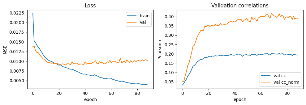
6. Fit

Defaults: MSE loss against the per-batch PSTH, AdamW + early stopping on val_cc_norm (Schoppe-style noise-corrected correlation across cells — see `metrics_paradigm.md <../docs/_source/md/metrics_paradigm.md>`__ §6.4).

With 6 train motifs the data is tiny; this typically converges within a minute or so on a single GPU. Don’t be surprised if the held-out cc is modest — the paper’s PSTH-decoding is an easier problem than predicting single-cell rate curves from clean spectrograms, and Le 2025’s noise ceiling on individual cells varies a lot.

optimizer = torch.optim.AdamW(model.parameters(), lr=2e-3, weight_decay=1e-4)

fitter = Fitter(
    model, train_loader, val_loader,
    optimizer=optimizer,
    device=device,
    max_epochs=120,
    patience=20,
    monitor='val_cc_norm',
    mode='max',
    log_fn=lambda d: print(
        f"epoch {d['epoch']:3d}  "
        f"train_loss={d['train_loss']:.4f}  "
        f"val_loss={d['val_loss']:.4f}  "
        f"val_cc_norm={torch.nanmean(d['val_cc_norm']):+.3f}",
        flush=True,
    ),
)
history = fitter.fit()
print(f'\nfinished after {len(history)} epochs')

epoch   0  train_loss=0.0223  val_loss=0.0137  val_cc_norm=+0.050
epoch   1  train_loss=0.0151  val_loss=0.0139  val_cc_norm=+0.052
epoch   2  train_loss=0.0148  val_loss=0.0128  val_cc_norm=+0.081
epoch   3  train_loss=0.0142  val_loss=0.0123  val_cc_norm=+0.106
epoch   4  train_loss=0.0136  val_loss=0.0122  val_cc_norm=+0.137
epoch   5  train_loss=0.0133  val_loss=0.0118  val_cc_norm=+0.151
epoch   6  train_loss=0.0127  val_loss=0.0113  val_cc_norm=+0.179
epoch   7  train_loss=0.0122  val_loss=0.0110  val_cc_norm=+0.207
epoch   8  train_loss=0.0116  val_loss=0.0106  val_cc_norm=+0.241
epoch   9  train_loss=0.0112  val_loss=0.0105  val_cc_norm=+0.246
epoch  10  train_loss=0.0108  val_loss=0.0101  val_cc_norm=+0.264
epoch  11  train_loss=0.0105  val_loss=0.0097  val_cc_norm=+0.287
epoch  12  train_loss=0.0102  val_loss=0.0097  val_cc_norm=+0.302
epoch  13  train_loss=0.0101  val_loss=0.0097  val_cc_norm=+0.314
epoch  14  train_loss=0.0100  val_loss=0.0094  val_cc_norm=+0.326
epoch  15  train_loss=0.0098  val_loss=0.0096  val_cc_norm=+0.325
epoch  16  train_loss=0.0096  val_loss=0.0093  val_cc_norm=+0.325
epoch  17  train_loss=0.0095  val_loss=0.0094  val_cc_norm=+0.348
epoch  18  train_loss=0.0093  val_loss=0.0095  val_cc_norm=+0.345
epoch  19  train_loss=0.0091  val_loss=0.0094  val_cc_norm=+0.351
epoch  20  train_loss=0.0090  val_loss=0.0092  val_cc_norm=+0.354
epoch  21  train_loss=0.0090  val_loss=0.0091  val_cc_norm=+0.347
epoch  22  train_loss=0.0089  val_loss=0.0093  val_cc_norm=+0.352
epoch  23  train_loss=0.0086  val_loss=0.0093  val_cc_norm=+0.353
epoch  24  train_loss=0.0085  val_loss=0.0092  val_cc_norm=+0.349
epoch  25  train_loss=0.0084  val_loss=0.0090  val_cc_norm=+0.359
epoch  26  train_loss=0.0083  val_loss=0.0093  val_cc_norm=+0.353
epoch  27  train_loss=0.0082  val_loss=0.0094  val_cc_norm=+0.352
epoch  28  train_loss=0.0080  val_loss=0.0092  val_cc_norm=+0.353
epoch  29  train_loss=0.0079  val_loss=0.0091  val_cc_norm=+0.363
epoch  30  train_loss=0.0079  val_loss=0.0099  val_cc_norm=+0.358
epoch  31  train_loss=0.0078  val_loss=0.0094  val_cc_norm=+0.360
epoch  32  train_loss=0.0076  val_loss=0.0093  val_cc_norm=+0.357
epoch  33  train_loss=0.0075  val_loss=0.0096  val_cc_norm=+0.359
epoch  34  train_loss=0.0073  val_loss=0.0094  val_cc_norm=+0.360
epoch  35  train_loss=0.0072  val_loss=0.0092  val_cc_norm=+0.367
epoch  36  train_loss=0.0070  val_loss=0.0092  val_cc_norm=+0.371
epoch  37  train_loss=0.0068  val_loss=0.0093  val_cc_norm=+0.375
epoch  38  train_loss=0.0067  val_loss=0.0092  val_cc_norm=+0.370
epoch  39  train_loss=0.0067  val_loss=0.0091  val_cc_norm=+0.374
epoch  40  train_loss=0.0067  val_loss=0.0098  val_cc_norm=+0.371
epoch  41  train_loss=0.0066  val_loss=0.0093  val_cc_norm=+0.374
epoch  42  train_loss=0.0064  val_loss=0.0094  val_cc_norm=+0.383
epoch  43  train_loss=0.0064  val_loss=0.0094  val_cc_norm=+0.383
epoch  44  train_loss=0.0064  val_loss=0.0094  val_cc_norm=+0.383
epoch  45  train_loss=0.0062  val_loss=0.0094  val_cc_norm=+0.384
epoch  46  train_loss=0.0062  val_loss=0.0097  val_cc_norm=+0.371
epoch  47  train_loss=0.0065  val_loss=0.0097  val_cc_norm=+0.379
epoch  48  train_loss=0.0064  val_loss=0.0101  val_cc_norm=+0.384
epoch  49  train_loss=0.0063  val_loss=0.0094  val_cc_norm=+0.392
epoch  50  train_loss=0.0061  val_loss=0.0093  val_cc_norm=+0.379
epoch  51  train_loss=0.0059  val_loss=0.0099  val_cc_norm=+0.374
epoch  52  train_loss=0.0057  val_loss=0.0096  val_cc_norm=+0.372
epoch  53  train_loss=0.0057  val_loss=0.0097  val_cc_norm=+0.398
epoch  54  train_loss=0.0056  val_loss=0.0094  val_cc_norm=+0.384
epoch  55  train_loss=0.0055  val_loss=0.0093  val_cc_norm=+0.389
epoch  56  train_loss=0.0055  val_loss=0.0095  val_cc_norm=+0.387
epoch  57  train_loss=0.0056  val_loss=0.0098  val_cc_norm=+0.374
epoch  58  train_loss=0.0056  val_loss=0.0097  val_cc_norm=+0.392
epoch  59  train_loss=0.0056  val_loss=0.0102  val_cc_norm=+0.396
epoch  60  train_loss=0.0056  val_loss=0.0096  val_cc_norm=+0.401
epoch  61  train_loss=0.0053  val_loss=0.0100  val_cc_norm=+0.400
epoch  62  train_loss=0.0052  val_loss=0.0098  val_cc_norm=+0.401
epoch  63  train_loss=0.0051  val_loss=0.0099  val_cc_norm=+0.401
epoch  64  train_loss=0.0050  val_loss=0.0097  val_cc_norm=+0.411
epoch  65  train_loss=0.0050  val_loss=0.0096  val_cc_norm=+0.414
epoch  66  train_loss=0.0048  val_loss=0.0098  val_cc_norm=+0.400
epoch  67  train_loss=0.0048  val_loss=0.0108  val_cc_norm=+0.390
epoch  68  train_loss=0.0049  val_loss=0.0095  val_cc_norm=+0.416
epoch  69  train_loss=0.0048  val_loss=0.0098  val_cc_norm=+0.409
epoch  70  train_loss=0.0047  val_loss=0.0101  val_cc_norm=+0.403
epoch  71  train_loss=0.0046  val_loss=0.0097  val_cc_norm=+0.403
epoch  72  train_loss=0.0045  val_loss=0.0104  val_cc_norm=+0.396
epoch  73  train_loss=0.0044  val_loss=0.0099  val_cc_norm=+0.400
epoch  74  train_loss=0.0044  val_loss=0.0097  val_cc_norm=+0.416
epoch  75  train_loss=0.0043  val_loss=0.0102  val_cc_norm=+0.398
epoch  76  train_loss=0.0042  val_loss=0.0097  val_cc_norm=+0.407
epoch  77  train_loss=0.0042  val_loss=0.0099  val_cc_norm=+0.402
epoch  78  train_loss=0.0042  val_loss=0.0102  val_cc_norm=+0.385
epoch  79  train_loss=0.0042  val_loss=0.0099  val_cc_norm=+0.397
epoch  80  train_loss=0.0042  val_loss=0.0101  val_cc_norm=+0.399
epoch  81  train_loss=0.0042  val_loss=0.0102  val_cc_norm=+0.393
epoch  82  train_loss=0.0041  val_loss=0.0100  val_cc_norm=+0.402
epoch  83  train_loss=0.0040  val_loss=0.0101  val_cc_norm=+0.398
epoch  84  train_loss=0.0040  val_loss=0.0104  val_cc_norm=+0.384
epoch  85  train_loss=0.0040  val_loss=0.0101  val_cc_norm=+0.401
epoch  86  train_loss=0.0040  val_loss=0.0104  val_cc_norm=+0.385
epoch  87  train_loss=0.0040  val_loss=0.0103  val_cc_norm=+0.393
epoch  88  train_loss=0.0039  val_loss=0.0102  val_cc_norm=+0.390

finished after 89 epochs

7. Training curves

epochs    = [h['epoch'] for h in history]
tr_loss   = [h['train_loss'] for h in history]
v_loss    = [h['val_loss'] for h in history]
v_cc      = [torch.nanmean(h['val_cc']).item() for h in history]
v_ccnorm  = [torch.nanmean(h['val_cc_norm']).item() for h in history]

fig, axs = plt.subplots(1, 2, figsize=(10, 3.5))
axs[0].plot(epochs, tr_loss, label='train', lw=1.5)
axs[0].plot(epochs, v_loss,  label='val',   lw=1.5)
axs[0].set_xlabel('epoch'); axs[0].set_ylabel('MSE'); axs[0].legend(); axs[0].set_title('Loss')
axs[1].plot(epochs, v_cc,     label='val cc',      lw=1.5)
axs[1].plot(epochs, v_ccnorm, label='val cc_norm', lw=1.5)
axs[1].set_xlabel('epoch'); axs[1].set_ylabel('Pearson r'); axs[1].legend()
axs[1].set_title('Validation correlations')
plt.tight_layout(); plt.show()

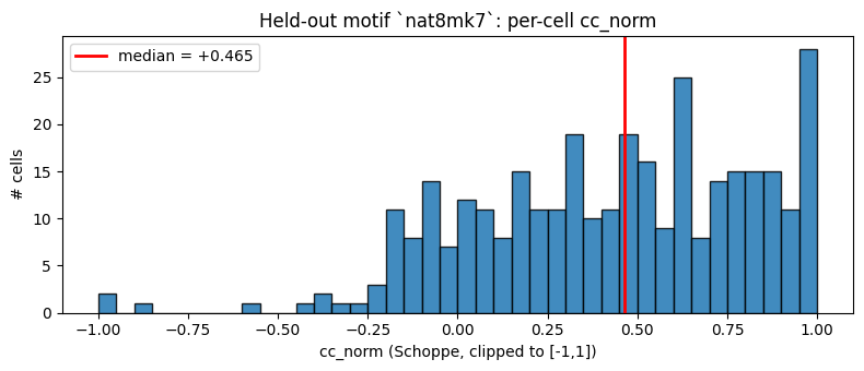
8. Test-set evaluation

On reading ``cc_norm``. Schoppe’s noise-corrected correlation divides the raw Pearson cc by the square root of the cell’s signal-power ratio (signal / total). For low-SNR cells with a single held-out motif, the denominator can land arbitrarily close to zero — so a handful of cells dominate the mean, while the median is robust. Report the median; clip the histogram to keep the visualization readable.

test_metrics = fitter.evaluate(test_loader)
test_cc      = test_metrics['cc'].cpu()
test_ccnorm  = test_metrics['cc_norm'].cpu()
print(f'test loss:       {test_metrics["loss"]:.4f}')
print(f'test cc       mean={torch.nanmean(test_cc):+.3f}   median={torch.nanmedian(test_cc):+.3f}')
print(f'test cc_norm  mean={torch.nanmean(test_ccnorm):+.3f}   median={torch.nanmedian(test_ccnorm):+.3f}')

# Clip the histogram view to [-1, 1] (a few low-SNR cells have cc_norm >> 1 due to ill-conditioned signal-power normalization).
clip = test_ccnorm.clamp(-1.0, 1.0).numpy()
fig, ax = plt.subplots(figsize=(8, 3.5))
ax.hist(clip, bins=40, range=(-1, 1), edgecolor='black', alpha=0.85)
ax.axvline(torch.nanmedian(test_ccnorm).item(), color='red', lw=2,
           label=f'median = {torch.nanmedian(test_ccnorm):+.3f}')
ax.set_xlabel('cc_norm (Schoppe, clipped to [-1,1])'); ax.set_ylabel('# cells')
ax.set_title(f'Held-out motif `{ds.stim_meta[C_stim_indices[test_iter[0]]]["motif"]}`: per-cell cc_norm')
ax.legend(); plt.tight_layout(); plt.show()

test loss:       0.0115
test cc       mean=+0.226   median=+0.183
test cc_norm  mean=+5.683   median=+0.465

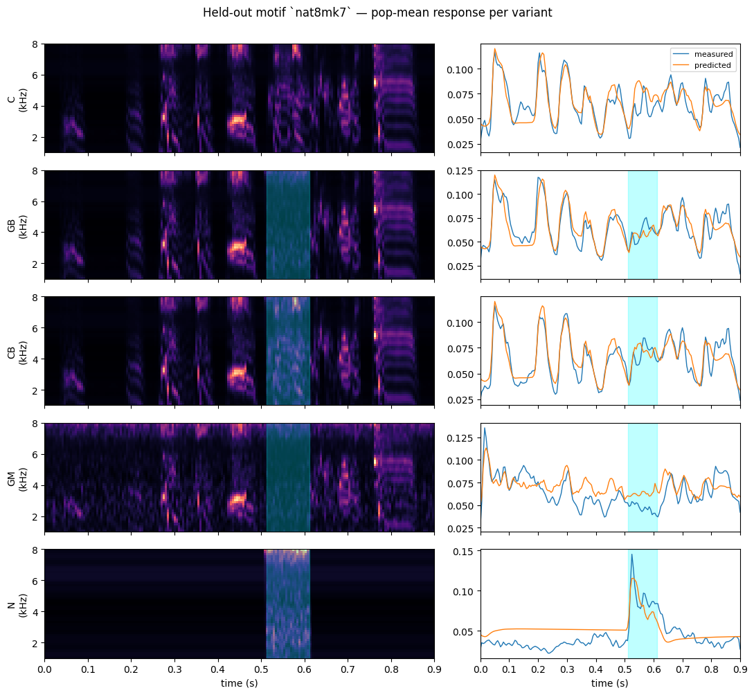
9. Bonus — model predictions on occluded variants

The fitted model only ever saw clean C stimuli. Pushing the held-out motif’s GB (Gap+Burst, illusion-inducing) and CB (Continuous+Burst, expected illusion) variants through it tells us how the model handles novel acoustic statistics outside its training distribution. This is not the paper’s restoration analysis (which works in PLS latent space across the whole population), but it’s a cheap qualitative sanity check.

ds.reset_stim_selection()
held_out_motif = ds.stim_meta[C_stim_indices[test_iter[0]]]['motif']
show_variants = ['C', 'GB', 'CB', 'GM', 'N']
show_ci = 1

fig, axs = plt.subplots(len(show_variants), 2, figsize=(11, 2.0*len(show_variants)),
                        sharex=True, gridspec_kw={'width_ratios': [3, 2]})
model.eval()
model.to(device)
with torch.no_grad():
    for row, variant in enumerate(show_variants):
        candidates = [i for i, m in enumerate(ds.stim_meta)
                      if m['motif'] == held_out_motif and m['variant'] == variant
                      and (m['critical_interval'] in (None, show_ci))]
        if not candidates:
            for ax in axs[row]:
                ax.set_visible(False)
            continue
        s_idx = candidates[0]
        meta = ds.stim_meta[s_idx]
        spec = ds.stims[s_idx]
        t = np.arange(spec.shape[-1]) * ds.dt * 1e-3
        # batch axis
        x = spec.unsqueeze(0).to(device)
        pred = model(x).cpu().squeeze(0).squeeze(1)  # (N, T)
        # ground truth on selected neurons
        resp = ds.responses[s_idx]
        psth = torch.stack([r.float().mean(0) if r.numel() > 1 else torch.full((spec.shape[-1],), float('nan'))
                            for r in resp])  # (N, T)
        # plot stim spectrogram
        axs[row, 0].imshow(spec[0].numpy(), aspect='auto', origin='lower', cmap='magma',
                           extent=[t[0], t[-1], ds.fmin/1000, ds.fmax/1000])
        if not np.isnan(meta['ci_onset_s']):
            axs[row, 0].axvspan(meta['ci_onset_s'], meta['ci_offset_s'], color='cyan', alpha=0.25)
        axs[row, 0].set_ylabel(f"{variant}\n(kHz)")
        # plot pop-mean predicted vs measured PSTH
        axs[row, 1].plot(t, psth.nanmean(0).numpy(), label='measured', lw=1.0)
        axs[row, 1].plot(t, pred.mean(0).numpy(),    label='predicted', lw=1.0)
        if not np.isnan(meta['ci_onset_s']):
            axs[row, 1].axvspan(meta['ci_onset_s'], meta['ci_offset_s'], color='cyan', alpha=0.25)
        if row == 0:
            axs[row, 1].legend(fontsize=8, loc='upper right')
axs[-1, 0].set_xlabel('time (s)'); axs[-1, 1].set_xlabel('time (s)')
fig.suptitle(f'Held-out motif `{held_out_motif}` — pop-mean response per variant', y=1.0)
plt.tight_layout(); plt.show()

Where to go next

• Leave-one-motif-out cross-validation — average cc / cc_norm across all 8 held-out motifs for a low-variance benchmark number.

• All variants in training — fit the encoding model on C + G + N +   CB + CM (the variants that contain no “information beyond the noise”) to give it more data and a wider acoustic distribution.

• Restoration metric — replicate the paper’s PLS / restoration-index pipeline in deepSTRF, contrasting GB vs CB trajectories in the model’s hidden state (rather than the recorded population). See select_restoration_quartet.

• synth8b — re-fit on the scrambled-syntax cohort; does cc_norm drop, as the paper’s restoration-index does?