Loading a pretrained model from the Hugging Face Hub

deepSTRF ships a curated set of pretrained checkpoints on the Hugging Face Hub. Loading one is a single line:

model = StateNet.from_pretrained("urancon/deepSTRF-statenet-gru-ns1")

This notebook walks through what that does under the hood, how to reproduce the published test metrics, and how to inspect the metadata we shipped alongside the weights. The full registry of pretrained models (and the recipes used to train them) lives in the docs: `pretrained_models.md <../docs/_source/md/pretrained_models.md>`__.

Setup — Google Colab

On Colab, install deepSTRF from source. On a local install (pip install -e .) this is a no-op.

import sys
if 'google.colab' in sys.modules:
    !pip install -q git+https://github.com/urancon/deepSTRF.git
    print("deepSTRF installed from GitHub.")
else:
    print("Local environment — assuming deepSTRF is already importable.")

Local environment — assuming deepSTRF is already importable.

Imports

%matplotlib inline
import matplotlib.pyplot as plt
import numpy as np
import torch
from torch.utils.data import DataLoader, Subset

from deepSTRF.datasets.audio.ns1 import NS1Dataset
from deepSTRF.metrics import corrcoef, normalized_corrcoef
from deepSTRF.models.audio import StateNet
from deepSTRF.utils import neural_collate, plot_psth_vs_pred

device = "cuda" if torch.cuda.is_available() else "cpu"
print(f"Using device: {device}")

Using device: cuda

1. Load the checkpoint

from_pretrained does three things behind the scenes:

1. Resolves the repo — if the argument is an existing local folder, it’s used directly; otherwise it’s treated as a Hub repo_id and downloaded into ~/.cache/huggingface/hub (idempotent + resumable).

2. Reads ``config.json`` — the architecture kwargs that were auto-captured when the model was constructed at training time, plus a _model_class sentinel for safety.

3. Calls ``StateNet(**config)`` then load_state_dict from model.safetensors.

The optional return_metadata=True also fetches the metadata.json blob we publish next to the weights (test metrics, training config, deepSTRF commit SHA used at training time).

REPO_ID = "urancon/deepSTRF-statenet-gru-ns1"

model, metadata = StateNet.from_pretrained(
    REPO_ID, map_location=device, return_metadata=True,
)
model.eval()

print(f"class:           {type(model).__name__}")
print(f"out_neurons:     {model.O}")
print(f"trainable params:{model.count_trainable_params():>9,}")

/home/ulysse/miniconda3/envs/deepstrf_dev/lib/python3.11/site-packages/tqdm/auto.py:21: TqdmWarning: IProgress not found. Please update jupyter and ipywidgets. See https://ipywidgets.readthedocs.io/en/stable/user_install.html
  from .autonotebook import tqdm as notebook_tqdm
Fetching 5 files: 100%|██████████| 5/5 [00:00<00:00, 15065.75it/s]

class:           StateNet
out_neurons:     119
trainable params:   39,081

2. Inspect the published metadata

Everything we know about the checkpoint at upload time is recorded in metadata. The same blob is the source of truth for the registry entry in `pretrained_models.md <../docs/_source/md/pretrained_models.md>`__.

import json
print(json.dumps(metadata, indent=2, sort_keys=True))

{
  "dataset": "NS1 (Harper et al. 2016, Rahman et al. 2020)",
  "library": "deepSTRF",
  "library_commit": "c07e561f7835454fdacbb35f38a8957668b8d1fd",
  "model_kwargs": {
    "connectivity": "LC",
    "hidden_channels": 7,
    "kernel_size": 7,
    "n_frequency_bands": 34,
    "rnn_type": "GRU",
    "stride": 3
  },
  "out_neurons": 119,
  "split": {
    "test_stim_idx": [
      17,
      18,
      19
    ],
    "train_stim_idx": [
      0,
      1,
      2,
      3,
      4,
      5,
      6,
      7,
      8,
      9,
      10,
      11,
      12,
      13
    ],
    "val_stim_idx": [
      14,
      15,
      16
    ]
  },
  "task": "audio neural response prediction",
  "test_metrics": {
    "cc_mean": 0.659480631351471,
    "cc_median": 0.681122899055481,
    "cc_norm_mean": 0.7703116536140442,
    "cc_norm_median": 0.7958264350891113,
    "loss": 0.015971951186656952
  },
  "training": {
    "device": "cuda",
    "epochs_run": 80,
    "fitter_kwargs": {
      "max_epochs": 80,
      "mode": "max",
      "monitor": "val_cc_norm",
      "patience": 15
    },
    "loss": "mse_loss vs PSTH",
    "optimizer": "AdamW",
    "optimizer_kwargs": {
      "lr": 0.001,
      "weight_decay": 0.0
    },
    "seed": 0,
    "train_time_min": 5.85
  }
}

3. Reproduce the test split

We auto-download NS1 and rebuild the same train/val/test stim split that was used at training time. The split indices are stored in metadata['split'], so any future change to the recipe is automatically reflected here.

ds = NS1Dataset(dt_ms=5.0, smooth=True, download=True)
test_idx = metadata['split']['test_stim_idx']
test_loader = DataLoader(Subset(ds, test_idx), batch_size=1,
                         shuffle=False, collate_fn=neural_collate)
print(f"NS1: {ds.N_neurons} cells, {len(ds.stims)} stims")
print(f"test stims: {test_idx}")

NS1: 119 cells, 20 stims
test stims: [17, 18, 19]

4. Run inference and compute test metrics

We run the canonical metrics from metrics_paradigm.md §6: per-cell Pearson cc against the trial-averaged PSTH, and Schoppe-style noise-corrected cc_norm against the full multi-trial response array. Both are NaN-aware so cells / timepoints with missing data don’t bias the average.

We then assert that the recomputed numbers match the ones we shipped in metadata — if they ever drift, something has changed in the dataset loader or the metrics that wasn’t accounted for at training time.

model.to(device)
preds, resps = [], []
with torch.no_grad():
    for stim, resp, mask, _ in test_loader:
        stim = stim.to(device)
        pred = model(stim)                          # (1, N, 1, T)
        preds.append(pred.cpu()); resps.append(resp.cpu())

# Concatenate along the BATCH axis — the canonical pattern from
# metrics_paradigm.md §7 / §11. normalized_corrcoef length-weights the
# signal-power estimate per stim, so each held-out stim must remain a
# distinct entry along dim 0 rather than getting time-glued into one
# long sequence.
pred_cat = torch.cat(preds, dim=0)        # (B=3, N, 1, T)
resp_cat = torch.cat(resps, dim=0)        # (B=3, N, R=20, T)

test_cc      = corrcoef(pred_cat, resp_cat, reduction='none')
test_cc_norm = normalized_corrcoef(pred_cat, resp_cat, method='schoppe', reduction='none')

summary = {
    'cc_mean':         float(torch.nanmean(test_cc)),
    'cc_median':       float(torch.nanmedian(test_cc)),
    'cc_norm_mean':    float(torch.nanmean(test_cc_norm)),
    'cc_norm_median':  float(torch.nanmedian(test_cc_norm)),
}
for k, v in summary.items():
    print(f"{k:>16s}: {v:+.4f}")

         cc_mean: +0.6595
       cc_median: +0.6811
    cc_norm_mean: +0.7703
  cc_norm_median: +0.7958

# Assert reproducibility against the published numbers.
expected = metadata['test_metrics']
for k, observed in summary.items():
    target = expected[k]
    diff = abs(observed - target)
    assert diff < 1e-3, (
        f"{k}: observed {observed:+.6f} vs published {target:+.6f} "
        f"(diff {diff:.2e}). Did the dataset loader change?"
    )
    print(f"{k:>16s}: observed {observed:+.4f}  vs  published {target:+.4f}  ✅")

         cc_mean: observed +0.6595  vs  published +0.6595  ✅
       cc_median: observed +0.6811  vs  published +0.6811  ✅
    cc_norm_mean: observed +0.7703  vs  published +0.7703  ✅
  cc_norm_median: observed +0.7958  vs  published +0.7958  ✅

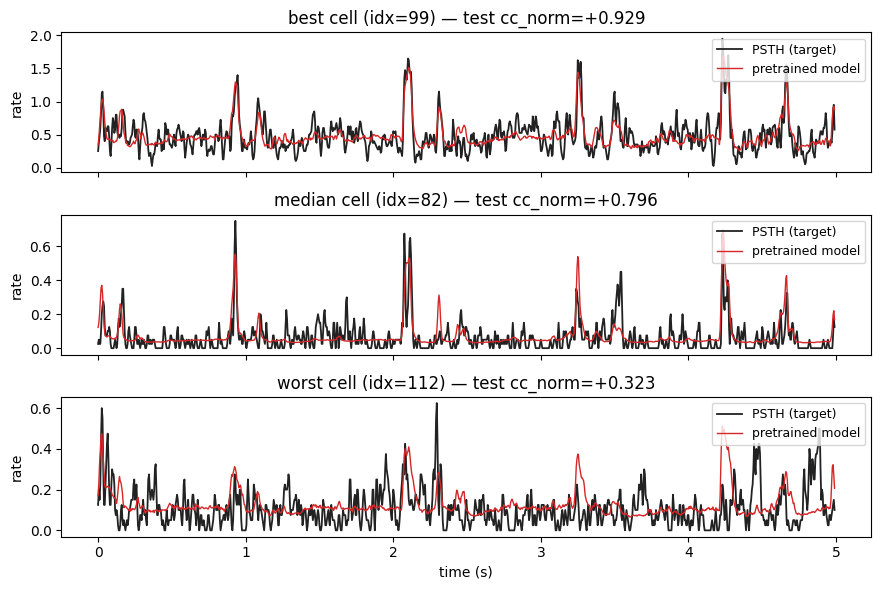
5. Visualise predictions

Pick the best, median, and worst cells (by test cc_norm) and overlay the model’s prediction on the trial-averaged response for one held-out stimulus.

ranking = test_cc_norm.argsort(descending=True)
best, median, worst = ranking[0].item(), ranking[len(ranking) // 2].item(), ranking[-1].item()
picks = [("best", best), ("median", median), ("worst", worst)]

# Run inference on the first held-out stim.
with torch.no_grad():
    stim0 = ds.stims[test_idx[0]].unsqueeze(0).to(device)
    pred0 = model(stim0).cpu().squeeze(0).squeeze(1)         # (N, T)
psth0 = torch.stack([r.mean(dim=0) for r in ds.responses[test_idx[0]]])

fig, axs = plt.subplots(3, 1, figsize=(9, 6), sharex=True)
for ax, (label, idx) in zip(axs, picks):
    plot_psth_vs_pred(
        psth0[idx], pred0[idx], dt_ms=5, ax=ax,
        title=f"{label} cell (idx={idx}) — test cc_norm={test_cc_norm[idx]:+.3f}",
        pred_label="pretrained model",
    )
axs[-1].set_xlabel("time (s)")
plt.tight_layout(); plt.show()

What’s next

• Browse the registry — `pretrained_models.md <../docs/_source/md/pretrained_models.md>`__ lists every checkpoint we publish, the architectures, training recipes, and test metrics. Each entry is reproducible from the recipe + the deepSTRF commit SHA recorded in its metadata.json on the Hub.

• Publish your own — after training, model.push_to_hub("your-name/your-model") is the upload counterpart to from_pretrained. You’ll need to be authenticated with hf auth login and have write access to the repo.

• Custom prefiltering — if your model used a non-JSON __init__ argument (e.g. an AdapTrans prefilter instance), pass it back via from_pretrained(..., extra_kwargs={'prefiltering': ...}). The saved config.json only stores JSON-serialisable kwargs.